Inference Review
May 19, 2025
Example Study
Fujiwara, Thomas, and Wantchekon, Leonard. “Can Informed Public Deliberation Overcome Clientelism? Experimental Evidence from Benin.”
SUMMARY: This paper studies the electoral effects of town hall meetings based on programmatic, nonclientelist platforms. The experiment involves the cooperation of leading candidates in a presidential election in Benin. A campaign strategy based solely on these meetings was assigned to randomly selected villages and compared to the standard strategy of clientelist rallies. We find that treatment reduces the prevalence of clientelism and does not affect turnout. Treatment also lowers the vote shares for the candidate with a political stronghold in the village and is more effective in garnering votes in regions where a candidate does not have a political stronghold.
Read in replication data
library (tidyverse)library (estimatr)library (haven)library (knitr)library (tidymodels)library (haven)<- read_dta ("data/survey_data_AEJ.dta" ) %>% mutate (treat = factor (treat)) %>% select (depcom, treat, index) %>% arrange (depcom)head (repData)
# A tibble: 6 × 3
  depcom treat  index
   <dbl> <fct>  <dbl>
1      1 0     -0.627
2      1 1     -0.513
3      2 0      0.137
4      2 1     -0.283
5     13 0     -0.170
6     13 1     -0.486
Examine Design
We have 24 villages, 12 in treatment and 12 in control.
# A tibble: 2 × 2
  treat     n
  <fct> <int>
1 0        12
2 1        12
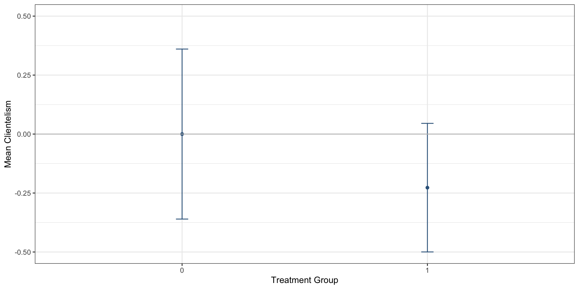
Means in treatment and control
%>% group_by (treat) %>% summarize (group_means = round (mean (index), 3 ))
# A tibble: 2 × 2
  treat group_means
  <fct>       <dbl>
1 0           0
2 1          -0.227
Calculate 95% CIs
First, estimate ATE and 95% CI
<- repData %>% group_by (treat) %>% summarize (mean = mean (index),sd = sd (index),se = sd/ sqrt (n ()- 1 ),conf.low = mean - 1.96 * se,conf.high = mean + 1.96 * se%>% select (treat, mean, conf.low, conf.high)
Interpretation
%>% kable (digits = 2 )
0
0.00
-0.36
0.36
1
-0.23
-0.50
0.05
Plot CIs
Code
library (lemon)%>% ggplot (., aes (y = mean, x = treat, ymin = conf.low, ymax = conf.high)) + geom_point (color = "steelblue4" ) + geom_errorbar (width = 0.05 , color = "steelblue4" ) + theme_bw () + labs (x = "Treatment Group" , y = "Mean Clientelism" ) + scale_y_symmetric (mid = 0 ) + geom_hline (yintercept = 0 , linetype = 1 , color = "grey" )
Treatment Effect Estimate
<- repData %>% specify (response = index, explanatory = treat) %>% calculate (stat = "diff in means" , order = c (1 , 0 ))
Response: index (numeric)
Explanatory: treat (factor)
# A tibble: 1 × 1
    stat
   <dbl>
1 -0.227
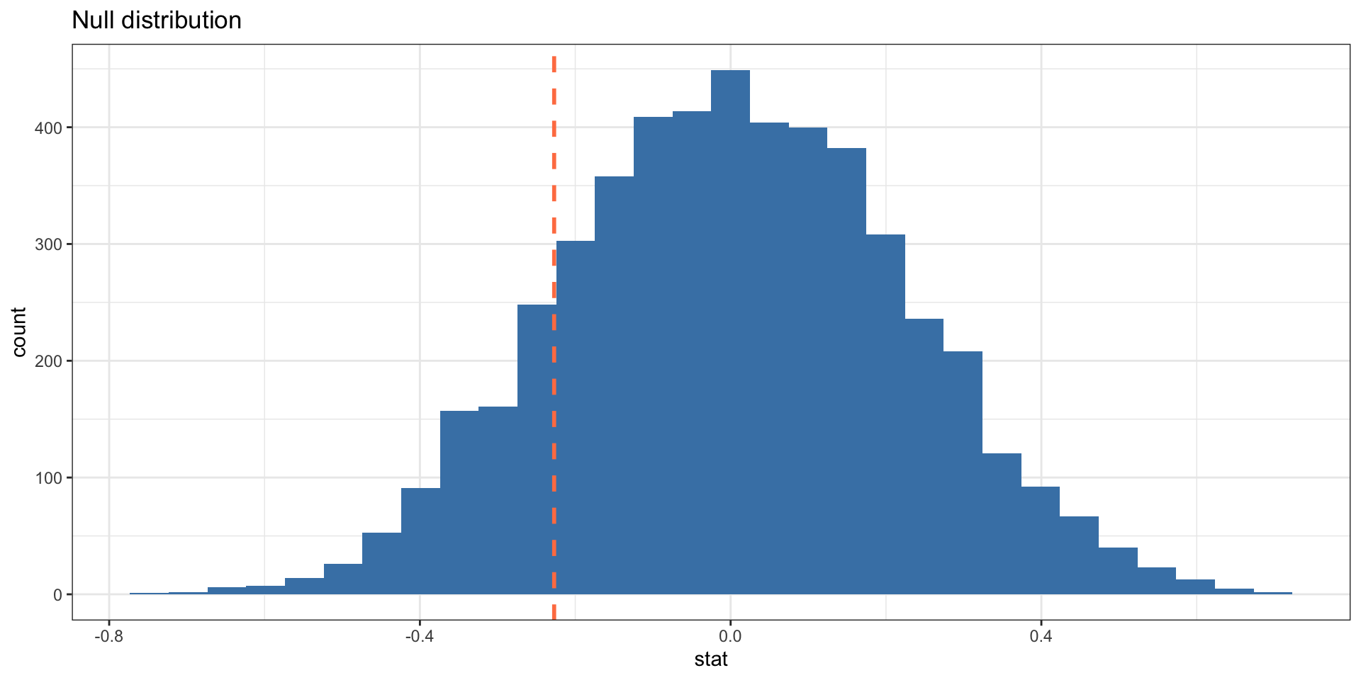
What will we do to test?
Reshuffle the treatment variable (permutation)
Calculate treatment effect
Repeat MANY times
Generates distribution of estimated treatment effects we would observe if the null hypothesis is true
Will use this distribution to see how likely we would be to observe our treatment effect, if the null hypothesis is true
Analysis
library (tidymodels)<- repData %>% specify (response = index, explanatory = treat)%>% hypothesize (null = "independence" ) %>% generate (5000 , type = "permute" ) %>% calculate (stat = "diff in means" , order = c ("1" , "0" ))
Plot
Calculate the p-value: single-tailed test
Prob of getting a value equal to or less than -0.2272066
mean (null_dist$ stat <= ate_estimate$ stat)
Calculate the p-value: two-tailed test
Probability of getting an ATE at least as large in absolute value than our actual estimate
mean (abs (null_dist$ stat) >= abs (ate_estimate$ stat))
Other approaches
Difference-in-means test
library (infer)%>% t_test (x = ., response = index, explanatory = treat, order = c (1 , 0 )) %>% select (estimate, p_value, lower_ci, upper_ci)
# A tibble: 1 × 4
  estimate p_value lower_ci upper_ci
     <dbl>   <dbl>    <dbl>    <dbl>
1   -0.227   0.315   -0.687    0.232
Other approaches
Using regression (our next topic!)
%>% lm_robust (formula = index ~ treat, data = .) %>% tidy () %>% select (term, estimate, p.value, conf.low, conf.high) %>% kable (digits = 2 )
(Intercept)
0.00
1.00
-0.37
0.37
treat1
-0.23
0.31
-0.68
0.23
Regression AND accounting for their research design
%>% lm_robust (formula = index ~ treat, fixed_effects = depcom, data = .) %>% tidy () %>% select (term, estimate, p.value, conf.low, conf.high) %>% kable (digits = 2 )
treat1
-0.23
0.02
-0.4
-0.05