Text Analysis
May 19, 2025
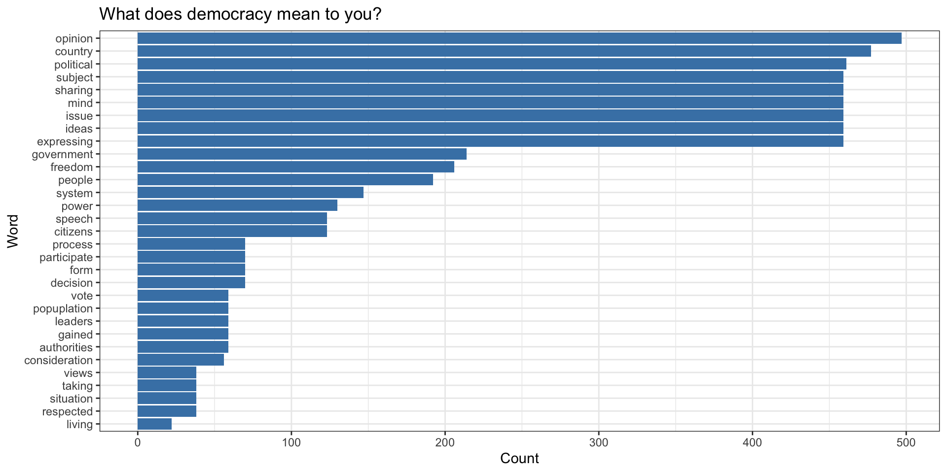
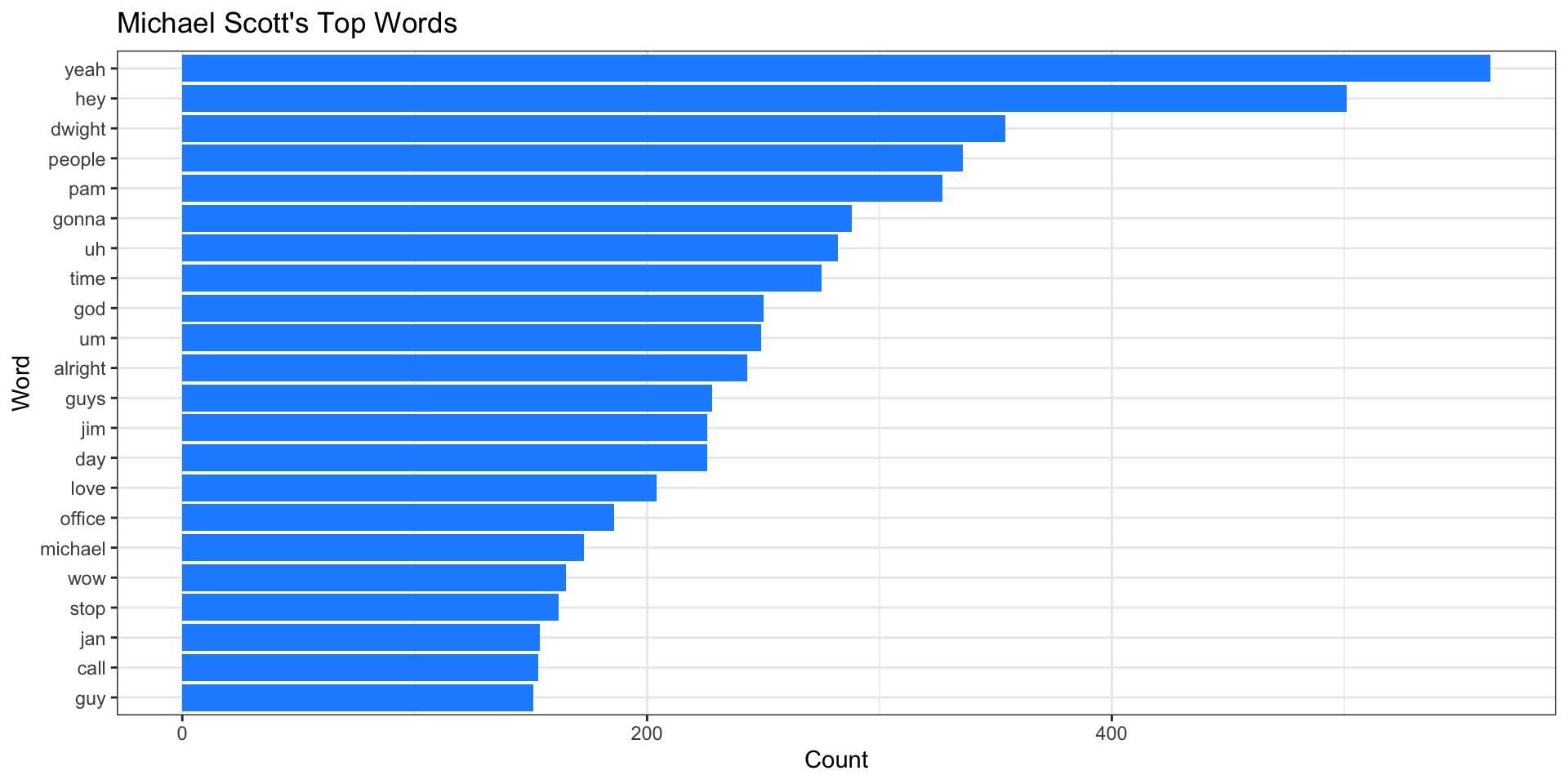
Top Words

Code to produce graph
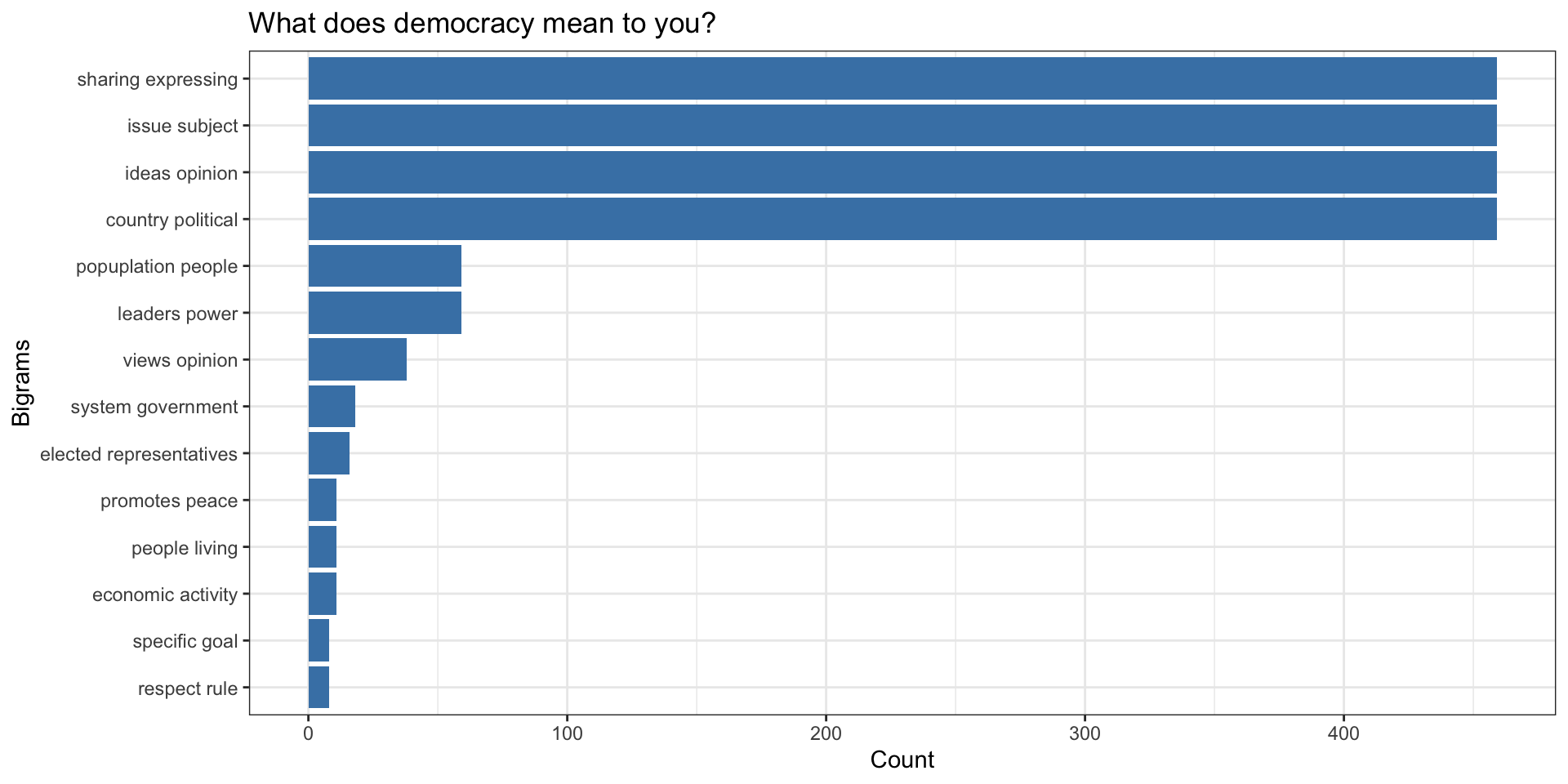
Top Bigrams
Word clouds
Code
library(wordcloud)
d <- unNest %>%
  filter(word != "NA") %>%
  filter(word != "government") %>%
  filter(word != "system") %>%
  filter(word != "political") %>%
    filter(word != "country") %>%
  count(word, sort = TRUE)  %>%  ungroup()
wordcloud(d$word, d$n, random.order = FALSE, max.words = 50, colors=brewer.pal(8,"Dark2"))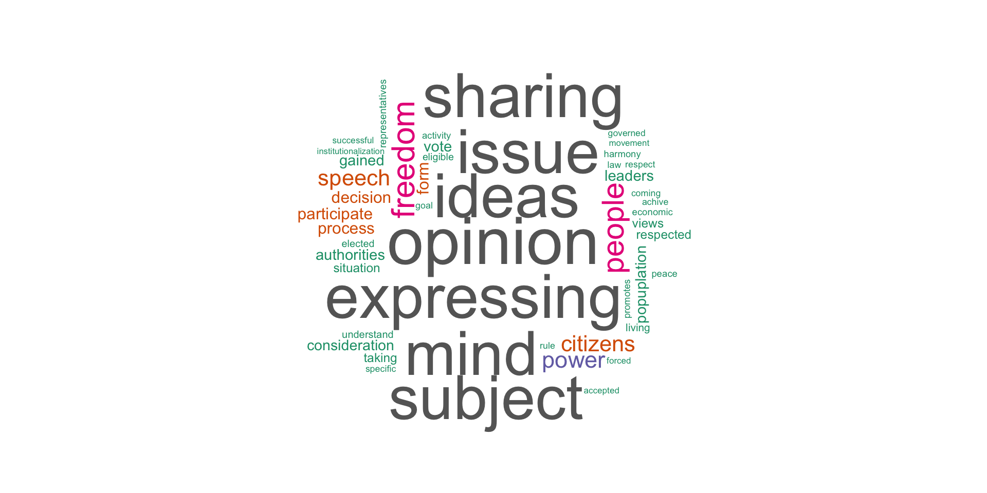
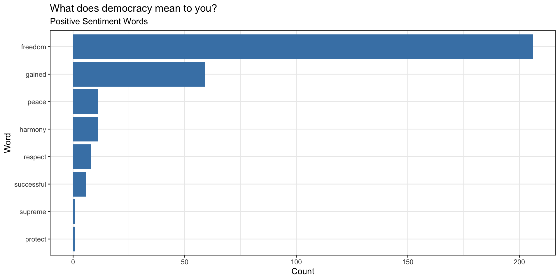
Common Words with Positive Sentiments
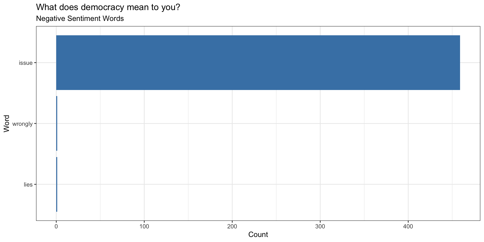
Common Words with Negative Sentiments
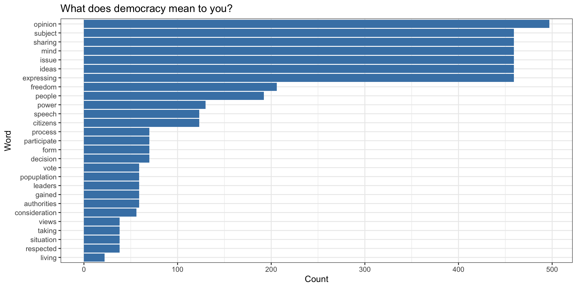
Top Words
N-Grams
Code
unNest_2 %>%
  filter(word != "NA") %>%
  count(word, sort = TRUE) %>%
  filter(n > 20) %>%
  mutate(word = reorder(word, n))%>%
  ggplot(aes(n, word)) +
    geom_col(fill = "steelblue") +
    theme_bw() +
    labs(x = "Count",
         y = "4-word phrase",
         title ="Michael Scott's Most Frequent Phrases",
         subtitle = "4 word N-grams")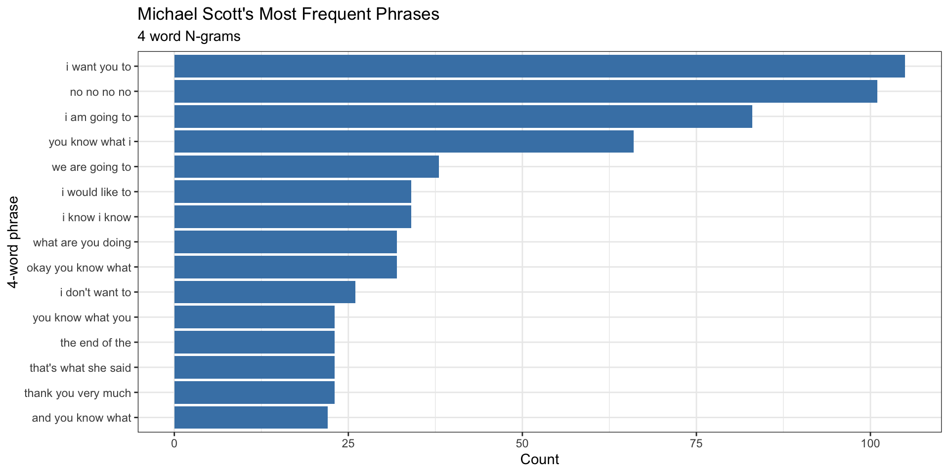
Most Common Positive Words
Code
scottBing %>%
  filter(word != "NA") %>%
  filter(sentiment == "positive") %>%
  count(word, sort = TRUE) %>%
  filter(n > 25) %>%
  mutate(word = reorder(word, n))%>%
  ggplot(aes(n, word)) +
    geom_col(fill = "dodgerblue") +
    theme_bw() +
    labs(x = "Count",
         y = "Word",
         title ="Michael Scott's Most Common Positive Words")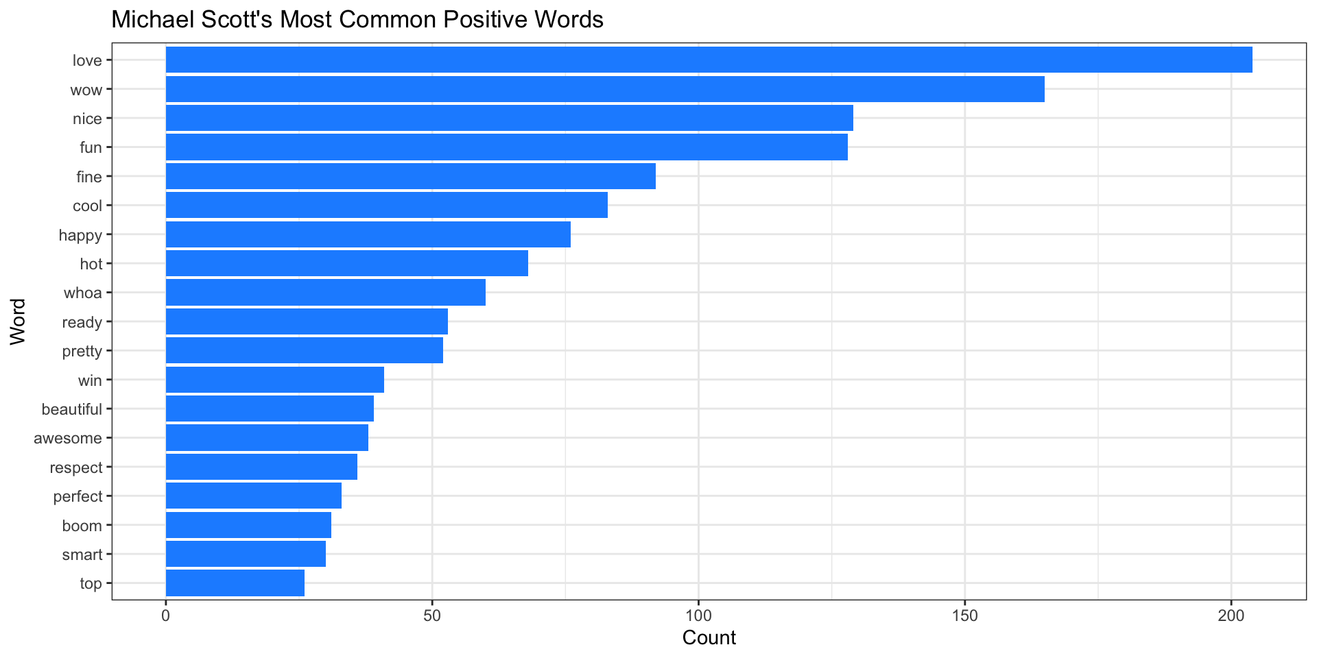
Most Common Negative Words
Code
scottBing %>%
  filter(word != "NA") %>%
  filter(sentiment == "negative") %>%
  count(word, sort = TRUE) %>%
  filter(n > 25) %>%
  mutate(word = reorder(word, n))%>%
  ggplot(aes(n, word)) +
    geom_col(fill = "darkred") +
    theme_bw() +
    labs(x = "Count",
         y = "Word",
         title =" Michael Scott's Most Common Negative Words")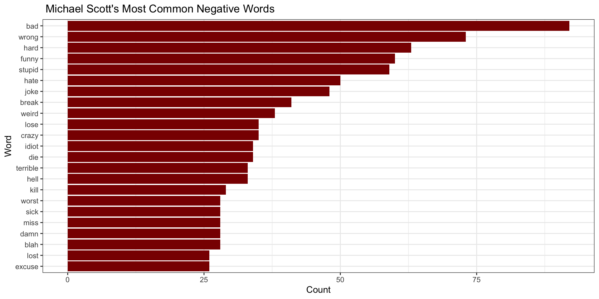
Posit Cloud
![]()