Multiple Regression
May 19, 2025
Load packages
Load VDEM Data
Linear Model with Multiple Predictors
Previously, we were interested in GDP per capita as a predictor of democracy.
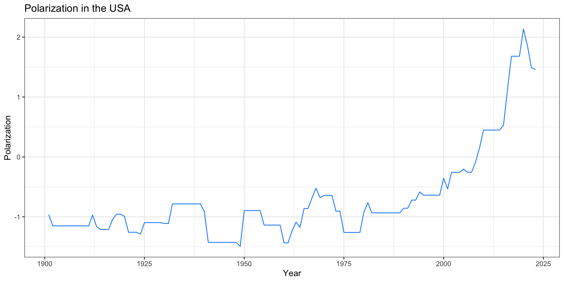
Now, let’s consider another predictor: polarization (also measured by V-Dem)
Polarization Measure in the USA
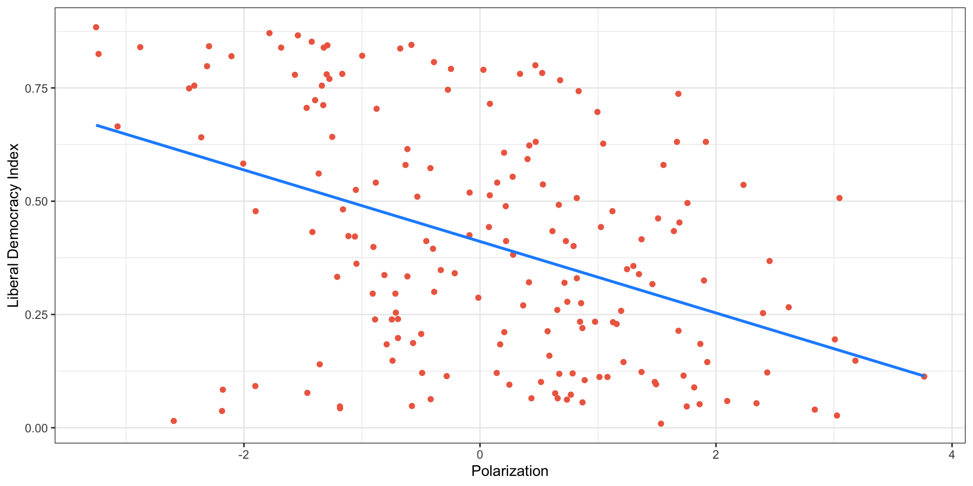
Polarization and Democracy in 2019

Model with Polarization as the only Predictor
How do we interpret the intercept and the slope estimate?
How are we figuring out what the “best” line is?
Model with Two Predictors
\[\hat{Y_i} = a + b_1*Polarization + b_2*GDPpc\]
OLS is searching for combination of \(a\), \(b_1\), and \(b_2\) that minimize sum of squared residuals
- same logic as model with one predictor, just more complicated
Model with Two Predictors
linear_reg() %>%
  set_engine("lm") %>%
  fit(v2x_libdem ~ v2cacamps + lg_gdppc, data = modelData) %>%
  tidy()
# A tibble: 3 × 5
term estimate std.error statistic p.value
<chr> <dbl> <dbl> <dbl> <dbl>
1 (Intercept) 0.182 0.0378 4.81 3.32e- 6
2 v2cacamps -0.0539 0.0120 -4.51 1.19e- 5
3 lg_gdppc 0.100 0.0147 6.82 1.50e-10Model with Two Predictors
\[\hat{Y_i} = a + b_1*Polarization + b_2*GDPpc\]
\[\hat{Y_i} = 0.18 + -0.05*Polarization + 0.10*GDPpc\]
Model with Two Predictors
\[\hat{Y_i} = a + b_1*Polarization + b_2*GDPpc\]
\[\hat{Y_i} = 0.18 + -0.05*Polarization + 0.10*GDPpc\]
- \(a\) is the predicted level of Y when BOTH GDP per capita and polarization are equal to 0
Model with Two Predictors
\[\hat{Y_i} = a + b_1*Polarization + b_2*GDPpc\]
\[\hat{Y_i} = 0.18 + -0.05*Polarization + 0.10*GDPpc\]
\(b_1\) is the impact of a 1-unit change in polarization on the predicted level of Y, holding GDP per capita fixed (all else equal)
- The relationship between polarization and democracy, controlling for GDP per capita.
Model with Two Predictors
\[\hat{Y_i} = a + b_1*Polarization + b_2*GDPpc\]
\[\hat{Y_i} = 0.18 + -0.05*Polarization + 0.10*GDPpc\]
- \(b_2\) is the impact of a 1-unit change in GDP per capita on the predicted level of Y, holding polarization fixed (all else equal)
Posit Cloud Practice
conflictData <- create_stateyears(system = 'gw') %>%
  filter(year %in% c(1946:1999)) %>%
  add_ucdp_acd(type=c("intrastate"), only_wars = FALSE) %>%
  add_democracy() %>% ## adds democracy measures
  add_creg_fractionalization() %>% ## adds ethnicity and religious fractionalization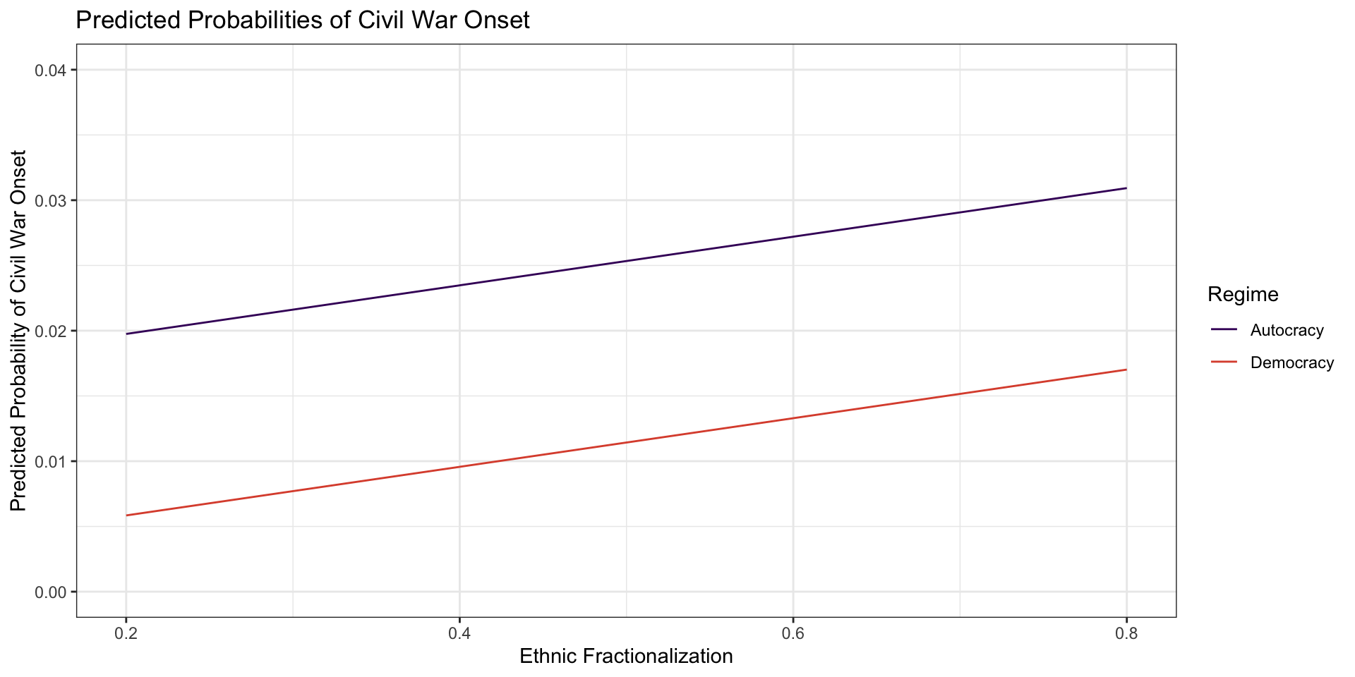
mutate(democracy = ifelse(v2x_polyarchy > .5, "Democracy", "Autocracy"))linear_reg() %>%
set_engine("lm") %>%
fit(ucdponset ~ democracy + ethfrac, data = conflictData) %>%
tidy()# A tibble: 3 × 5
term estimate std.error statistic p.value
<chr> <dbl> <dbl> <dbl> <dbl>
1 (Intercept) 0.0160 0.00364 4.40 0.0000111
2 democracyDemocracy -0.0139 0.00398 -3.50 0.000475
3 ethfrac 0.0186 0.00651 2.86 0.00425 What is predicted probability of civil war onset for a country that is a democracy and has an ethfrac score of 0.5?
Save model as an object
Remove the tidy() so it is saved as a model object
- Create new data frame for prediction
- Use
predict()to generate predicted values
- For a non-democracy, how does the predicted probability of civil war onset change if
ethfracchanged from 0.25 to 0.75?
Plot Predicted Values from Model
predData3 <- data.frame(democracy = c("Autocracy", "Autocracy", "Autocracy", "Autocracy",
                        "Democracy", "Democracy", "Democracy", "Democracy"),
                       ethfrac = c(.2, .4, .6,  .8,
                                    .2, .4, .6, .8)
                       )
predData3
democracy ethfrac
1 Autocracy 0.2
2 Autocracy 0.4
3 Autocracy 0.6
4 Autocracy 0.8
5 Democracy 0.2
6 Democracy 0.4
7 Democracy 0.6
8 Democracy 0.8Plot Predicted Values from Model
  democracy ethfrac       .pred
1 Autocracy     0.2 0.019751861
2 Autocracy     0.4 0.023477869
3 Autocracy     0.6 0.027203877
4 Autocracy     0.8 0.030929885
5 Democracy     0.2 0.005843543
6 Democracy     0.4 0.009569551
7 Democracy     0.6 0.013295559
8 Democracy     0.8 0.017021567
Plot Predicted Values from Model
Code
ggplot(plotData, aes(x = ethfrac, y = .pred, color = democracy)) +
  geom_line() + theme_bw() + labs(x = "Ethnic Fractionalization",
  y = "Predicted Probability of Civil War Onset", color = "Regime",
  title = "Predicted Probabilities of Civil War Onset") + scale_color_viridis_d(option = "B", begin = .2, end = .6) + ylim(0, 0.04)