Interaction Models
May 19, 2025
Load packages
Multiple Predictors: Interaction Models
Example: Oil Wealth and Democracy
What is the political resource curse?
Set up data: Use the year 2005
Distribution of Oil Wealth per Capita
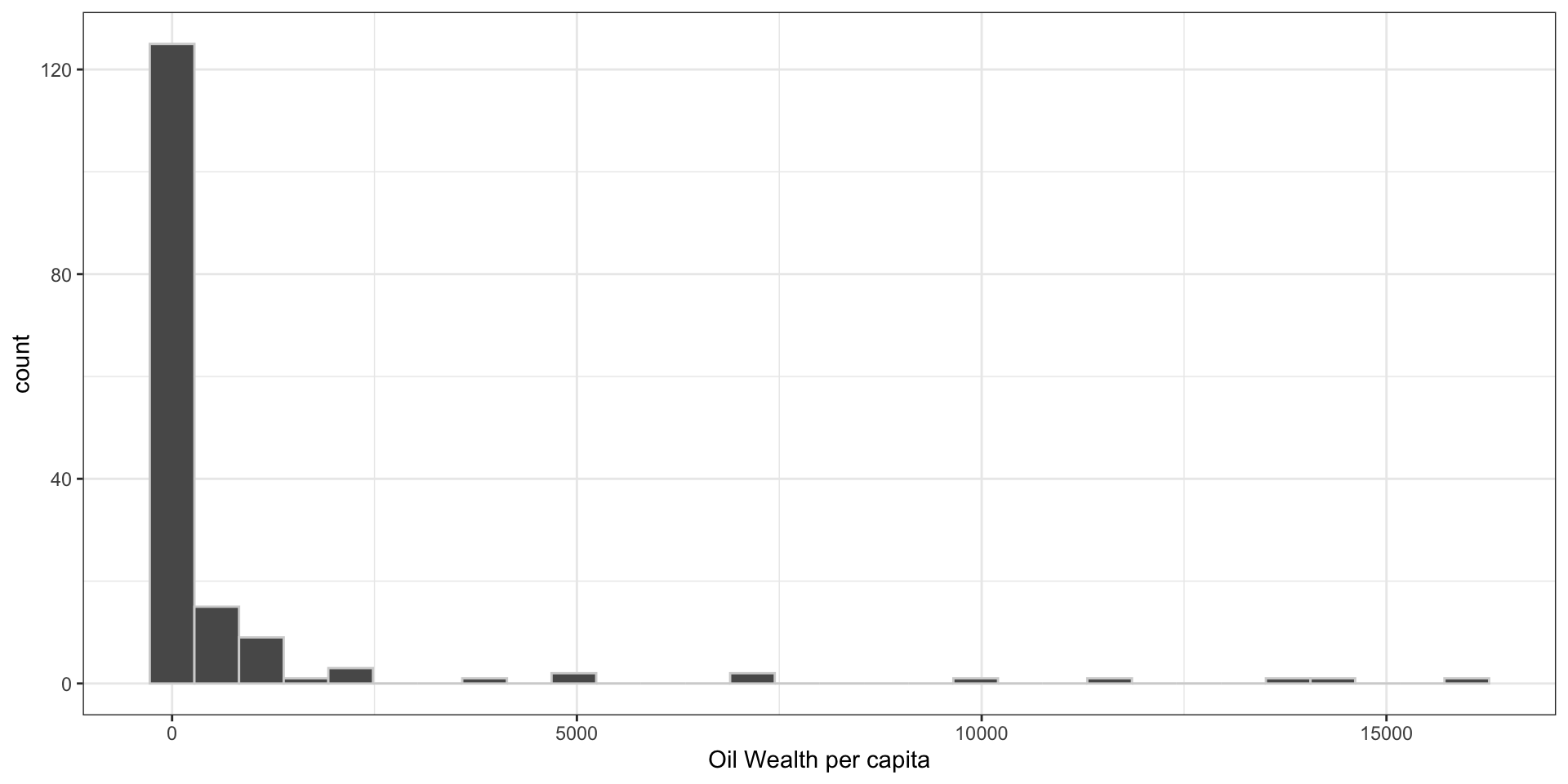
Create a Dummy Variable for High Oil Wealth
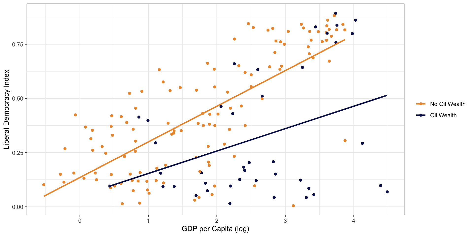
Democracy, GDP, and Oil
How should we interpret this graph?
Model with Oil and GDP per Capita, No Interaction
What is correct interpretation of these results?
# A tibble: 3 × 5
  term          estimate std.error statistic  p.value
  <chr>            <dbl>     <dbl>     <dbl>    <dbl>
1 (Intercept)      0.157    0.0318      4.95 1.84e- 6
2 lg_gdppc         0.152    0.0143     10.6  3.25e-20
3 oilOil Wealth   -0.234    0.0394     -5.93 1.85e- 8
Interaction Model
- Question: Does GDP per capita have a different relationship to democracy in Oil rich versus non-Oil rich countries?
Interaction Model
\(Y_i = a + b_1*GDPpc + b_2*Oil + b_3*GDPpc*Oil\)
- \(b_3*GDPpc*OilWealth\) captures the interaction
Interaction Model: Interpretation
- How should we interpret \(a\)?
\(Y_i = a + b_1*GDPpc + b_2*Oil + b_3*GDPpc*Oil\)
- \(a\) is predicted level of democracy where GDPpc = 0 and Oil Wealth = 0
Interaction Model: Interpretation
What happens if we set Oil Wealth to 0?
\(Y_i = a + b_1 * GDPpc + b_2 * Oil + b_3 * GDPpc * Oil\)
\(Y_i = a + b_1 * GDPpc + b_2 * 0 + b_3 * GDPpc * 0\)
\(Y_i = a + b_1 * GDPpc\)
- \(b_1\) is the association between GDP per capita and democracy, when oil wealth = 0
Interaction Model: Interpretation
What happens if we set GDPpc to 0?
\(Y_i = a + b_1 * GDPpc + b_2 * Oil + b_3 * GDPpc * Oil\)
\(Y_i = a + b_1 * 0 + b_2 * Oil + b_3 * Oil * 0\)
\(Y_i = a + b_2 * Oil\)
\(b_2\) is the association between oil and democracy, when GDP per capita = 0
Interaction Model: Interpretation
- What happens if we set Oil Wealth to 1?
\(Y_i = a + b_1 * GDPpc + b_2 * 1 + b_3 * GDPpc * 1\)
\(Y_i = a + b_1 * GDPpc + b_2 + b_3 * GDPpc\)
Rearrange: \(Y_i = a + (b_1 + b_3) * GDPpc + b_2\)
Interaction Model: Interpretation
\(Y_i = a + (b_1 + b_3) * GDPpc + b_2\)
\(b_1 + b_3\) is the association between GDP per capita and democracy, when oil wealth = 1
\(b_3\) is the difference in the association between GDP per capita and democracy for high oil wealth versus low oil wealth countries.
Run the Interaction Model
# A tibble: 4 × 5
  term                   estimate std.error statistic  p.value
  <chr>                     <dbl>     <dbl>     <dbl>    <dbl>
1 (Intercept)              0.135     0.0341     3.97  1.10e- 4
2 lg_gdppc                 0.164     0.0160    10.3   2.33e-19
3 oilOil Wealth           -0.0848    0.0949    -0.894 3.73e- 1
4 lg_gdppc:oilOil Wealth  -0.0609    0.0354    -1.72  8.70e- 2
Interpretation
\(\hat{Y_i}\) = .138 + .164 * \(GDPpc_i\) + (-0.085) * \(Oil_i\) + (-0.0607) * \(GDPpc_i\) * \(Oil_i\)
Relationship between GDP and democracy without oil: \(0.164\)
Relationship with oil: \(0.164 -0.0607 = 0.1033\)
Conclusion?
Wealth predicts greater democracy, but to a lesser degree when that wealth is driven by oil wealth
Is this difference due to chance?
Does GDP have a lower relationship to democracy in oil rich countries?
Is 0.164 without oil different from 0.1033 with oil?
- What is the null hypothesis? What is the alternative?
Is this difference due to chance?
We can interpret the p-value in the same way as we learned previously. Same with the 95 percent confidence intervals.
# A tibble: 4 × 6
  term                   estimate std.error p.value conf.low conf.high
  <chr>                     <dbl>     <dbl>   <dbl>    <dbl>     <dbl>
1 (Intercept)               0.135     0.034   0        0.068     0.202
2 lg_gdppc                  0.164     0.016   0        0.133     0.196
3 oilOil Wealth            -0.085     0.095   0.373   -0.272     0.103
4 lg_gdppc:oilOil Wealth   -0.061     0.035   0.087   -0.131     0.009
Is this difference due to chance?
95% Confidence Interval: [-0.131, 0.009]: mostly negative
p-value of interaction term: 0.089
- this is higher that 0.05, but close and remember that the cutoff is arbitrary
Questions?
Another Example: Resume Experiement
Is gender discrimination in call backs different for those with or without a college degree?
Fit interaction model
library(openintro)
linear_reg() %>%
  set_engine("lm") %>%
  fit(received_callback ~ gender*college_degree, data = resume) %>%
  tidy()
# A tibble: 4 × 5
term estimate std.error statistic p.value
<chr> <dbl> <dbl> <dbl> <dbl>
1 (Intercept) 0.0796 0.00775 10.3 1.71e-24
2 genderm 0.0463 0.0247 1.88 6.04e- 2
3 college_degree 0.00429 0.00946 0.453 6.51e- 1
4 genderm:college_degree -0.0635 0.0267 -2.38 1.74e- 2# A tibble: 4 × 5
term estimate std.error statistic p.value
<chr> <dbl> <dbl> <dbl> <dbl>
1 (Intercept) 0.0796 0.00775 10.3 1.71e-24
2 genderm 0.0463 0.0247 1.88 6.04e- 2
3 college_degree 0.00429 0.00946 0.453 6.51e- 1
4 genderm:college_degree -0.0635 0.0267 -2.38 1.74e- 2\(\hat{Y_i}\) = .08 + .05 * \(M_i\) + 0.004 * \(Coll_i\) + (-0.06) * \(M_i\) * \(Coll_i\)
\(\hat{Y_i}\) = .08 + .05 * \(M_i\) + 0.004 * \(Coll_i\) -0.06 * \(M_i\) * \(Coll_i\)
What is the predicted impact of being male (relative to female) for people without a college degree (\(Coll_i = 0\))?
0.05 increase in the probability of getting a call back
\(\hat{Y_i}\) = .08 + .05 * \(M_i\) + 0.004 * \(Coll_i\) -0.06 * \(M_i\) * \(Coll_i\)
What is the impact of being male (relative to female) for people with a college degree (\(Coll_i = 1\))?
0.05 + (-0.06) = -0.01 = 0.01 decrease in the probability of getting a call back
\(\hat{Y_i}\) = .08 + .05 * \(M_i\) + 0.004 * \(Coll_i\) -0.06 * \(M_i\) * \(Coll_i\)
What is the predicted call back rate for women without a college degree?
The intercept!
\(\hat{Y_i}\) = .08 + .05 * 0 + 0.004 * 0 + (-0.06) * 0 * 1 = 0.08 + 0.004 = 0.08
\(\hat{Y_i}\) = .08 + .05 * \(M_i\) + 0.004 * \(Coll_i\) -0.06 * \(M_i\) * \(Coll_i\)
What is the predicted call back rate for men without a college degree?
\(\hat{Y_i}\) = .08 + .05 * 1 + 0.004 * 0 + (-0.06) * 0 * 1 = 0.08 + 0.05 = 0.13
\(\hat{Y_i}\) = .08 + .05 * \(M_i\) + 0.004 * \(Coll_i\) -0.06 * \(M_i\) * \(Coll_i\)
What is the predicted call back rate value for men with a college degree?
\(\hat{Y_i}\) = .08 + .05 * 1 + 0.004 * 1 + (-0.06) * 1 * 1 = 0.074
\(\hat{Y_i}\) = .08 + .05 * \(M_i\) + 0.004 * \(Coll_i\) -0.06 * \(M_i\) * \(Coll_i\)
What is the predicted call back rate for women with a college degree?
\(\hat{Y_i}\) = .08 + .05 * 0 + 0.004 * 1 + (-0.06) * 0 * 1 = 0.08 + 0.004 = 0.084
Inference
Is the difference in gender discrimination in the two education groups likely to have happened due to chance?
What is the null hypothesis? The alternative?
Inference
# A tibble: 4 × 6
  term                   estimate std.error p.value conf.low conf.high
  <chr>                     <dbl>     <dbl>   <dbl>    <dbl>     <dbl>
1 (Intercept)               0.08      0.008   0        0.064     0.095
2 genderm                   0.046     0.025   0.06    -0.002     0.095
3 college_degree            0.004     0.009   0.651   -0.014     0.023
4 genderm:college_degree   -0.063     0.027   0.017   -0.116    -0.011
p-value is 0.0174: we would reject the null hypothesis of no difference
Conclusion: The impact of being male relative to female on call back rates is different for those with and without a college degree.