Rows: 4,870
Columns: 30
$ job_ad_id              <dbl> 384, 384, 384, 384, 385, 386, 386, 385, 386, 38…
$ job_city               <chr> "Chicago", "Chicago", "Chicago", "Chicago", "Ch…
$ job_industry           <chr> "manufacturing", "manufacturing", "manufacturin…
$ job_type               <chr> "supervisor", "supervisor", "supervisor", "supe…
$ job_fed_contractor     <dbl> NA, NA, NA, NA, 0, 0, 0, 0, 0, 0, 0, 0, 0, 0, N…
$ job_equal_opp_employer <dbl> 1, 1, 1, 1, 1, 1, 1, 1, 1, 1, 1, 1, 1, 1, 1, 1,…
$ job_ownership          <chr> "unknown", "unknown", "unknown", "unknown", "no…
$ job_req_any            <dbl> 1, 1, 1, 1, 1, 0, 0, 1, 0, 0, 1, 1, 1, 1, 0, 0,…
$ job_req_communication  <dbl> 0, 0, 0, 0, 0, 0, 0, 0, 0, 0, 0, 0, 1, 1, 0, 0,…
$ job_req_education      <dbl> 0, 0, 0, 0, 0, 0, 0, 0, 0, 0, 0, 0, 0, 0, 0, 0,…
$ job_req_min_experience <chr> "5", "5", "5", "5", "some", "", "", "some", "",…
$ job_req_computer       <dbl> 1, 1, 1, 1, 1, 0, 0, 1, 0, 0, 1, 1, 1, 1, 0, 0,…
$ job_req_organization   <dbl> 0, 0, 0, 0, 1, 0, 0, 1, 0, 0, 0, 0, 1, 1, 0, 0,…
$ job_req_school         <chr> "none_listed", "none_listed", "none_listed", "n…
$ received_callback      <dbl> 0, 0, 0, 0, 0, 0, 0, 0, 0, 0, 0, 0, 0, 0, 0, 0,…
$ firstname              <chr> "Allison", "Kristen", "Lakisha", "Latonya", "Ca…
$ race                   <chr> "white", "white", "black", "black", "white", "w…
$ gender                 <chr> "f", "f", "f", "f", "f", "m", "f", "f", "f", "m…
$ years_college          <int> 4, 3, 4, 3, 3, 4, 4, 3, 4, 4, 4, 4, 4, 4, 4, 1,…
$ college_degree         <dbl> 1, 0, 1, 0, 0, 1, 1, 0, 1, 1, 1, 1, 1, 1, 1, 0,…
$ honors                 <int> 0, 0, 0, 0, 0, 1, 0, 0, 0, 0, 0, 0, 0, 0, 0, 0,…
$ worked_during_school   <int> 0, 1, 1, 0, 1, 0, 1, 0, 0, 1, 0, 1, 0, 1, 0, 0,…
$ years_experience       <int> 6, 6, 6, 6, 22, 6, 5, 21, 3, 6, 8, 8, 4, 4, 5, …
$ computer_skills        <int> 1, 1, 1, 1, 1, 0, 1, 1, 1, 0, 1, 1, 1, 1, 0, 1,…
$ special_skills         <int> 0, 0, 0, 1, 0, 1, 1, 1, 1, 1, 1, 0, 1, 0, 1, 1,…
$ volunteer              <int> 0, 1, 0, 1, 0, 0, 1, 1, 0, 1, 1, 0, 0, 0, 1, 0,…
$ military               <int> 0, 1, 0, 0, 0, 0, 0, 0, 0, 0, 0, 0, 0, 0, 0, 0,…
$ employment_holes       <int> 1, 0, 0, 1, 0, 0, 0, 1, 0, 0, 1, 0, 1, 0, 0, 0,…
$ has_email_address      <int> 0, 1, 0, 1, 1, 0, 1, 1, 0, 1, 1, 1, 0, 0, 1, 0,…
$ resume_quality <chr> "low", "high", "low", "high", "high", "low", "h…Logistic Regression
Classification
May 19, 2025
Review
Review
- True or False: When the coefficient on a predictor is statistically significant, we have proved that the predictor has a causal impact on the outcome?
- False: The answer depends on the research design.
Review
- True or False: When the coefficient on a predictor is statistically significant, we have proved that the predictor has large and important association with outcome?
- False: The answer depends on your substantive interpretation of the effect sizes and on your knowledge of the specific issue.
Models with Binary (0/1) Outcomes
Binary Outcomes
So far we have looked at continuous or numerical outcomes (response variables)
We are often also interested in outcome variables that are binary (Yes/No, or 0/1)
- Did violence happen, or not?
- Classification: is this email spam?
Racial Discrimination Study
Bertrand and Mullainathan (2003)
data are in openintro package
Racial Discrimination Study
Outcome variable: Applicant received call back (yes=1, No=0)
Predictors:
- Race of applicant (randomly assigned)
- Years of Experience
Racial Discrimination Study
# A tibble: 2 × 2
  race  callRate
  <chr>    <dbl>
1 black   0.0645
2 white   0.0965
Racial Discrimination Study
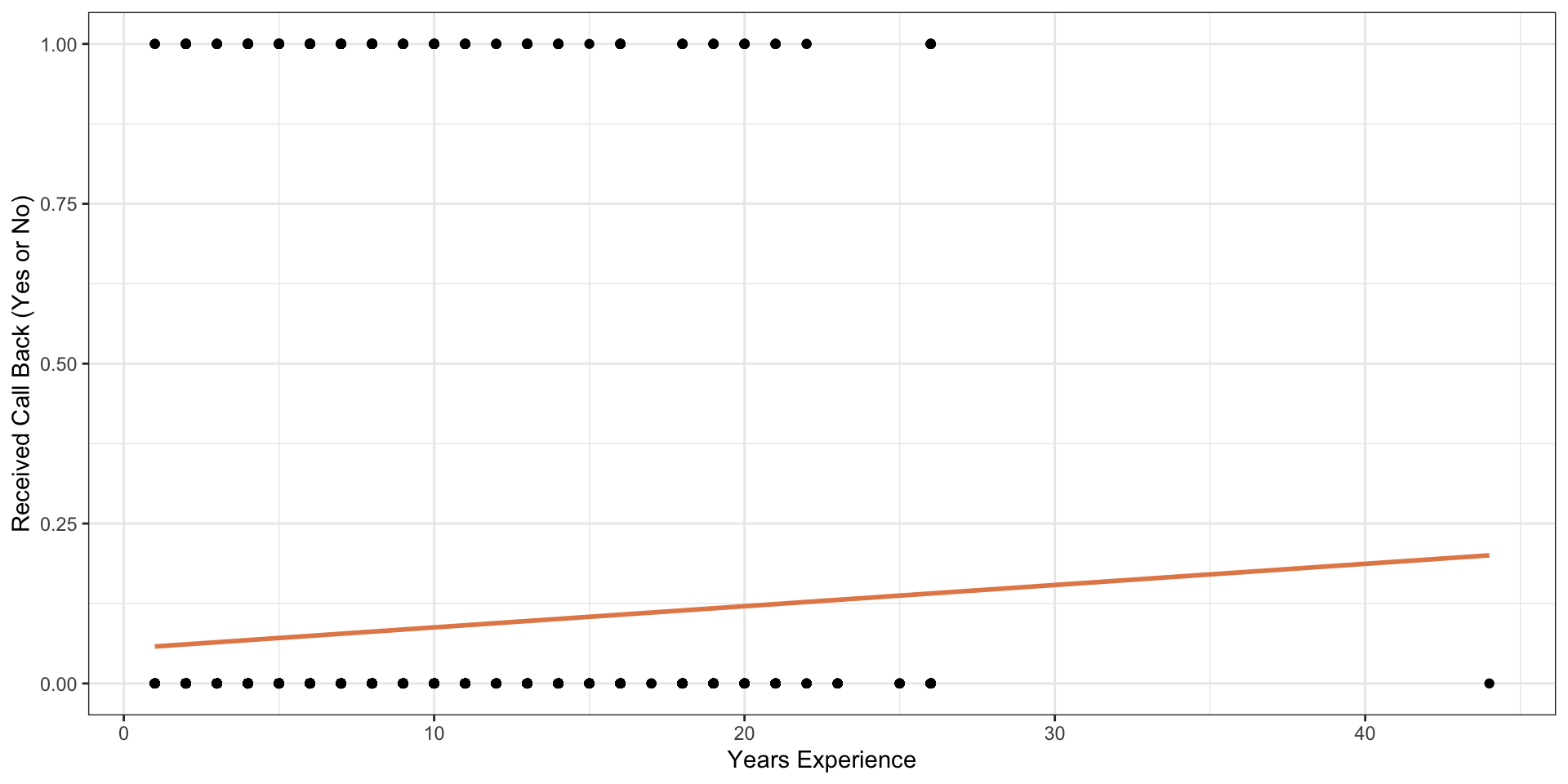
Racial Discrimination Study

Racial Discrimination Study
We want a model to predict call backs: our linear models do not really work in this situation
Modeling
We can treat each outcome (call back or not) as successes and failures arising from separate Bernoulli trials
- Bernoulli trial: a random experiment with exactly two possible outcomes, “success” and “failure”, in which the probability of success is the same every time the experiment is conducted
Modeling
- Each Bernoulli trial can have a separate probability of success
\[ y_i ∼ Bern(p) \]
Modeling
We can then use the predictor variables to model that probability of success, \(p_i\)
We can’t use a linear model for \(p_i\) (since \(p_i\) must be between 0 and 1) but we can transform the linear model to have the appropriate range
Generalized linear models
This is a very general way of addressing many problems in regression and the resulting models are called generalized linear models (GLMs)
Logistic regression is a very common example
GLMs
All GLMs have the following three characteristics:
- A probability distribution describing a generative model for the outcome variable
- A linear model: \[\eta = \beta_0 + \beta_1 X_1 + \cdots + \beta_k X_k\]
- A link function that relates the linear model to the parameter of the outcome distribution
Logistic regression
Logistic regression is a GLM used to model a binary categorical outcome (0 or 1)
In logistic regression, the link function that connects \(\eta_i\) to \(p_i\) is the logit function
Logit function: For \(0\le p \le 1\)
\[logit(p) = \log\left(\frac{p}{1-p}\right)\]
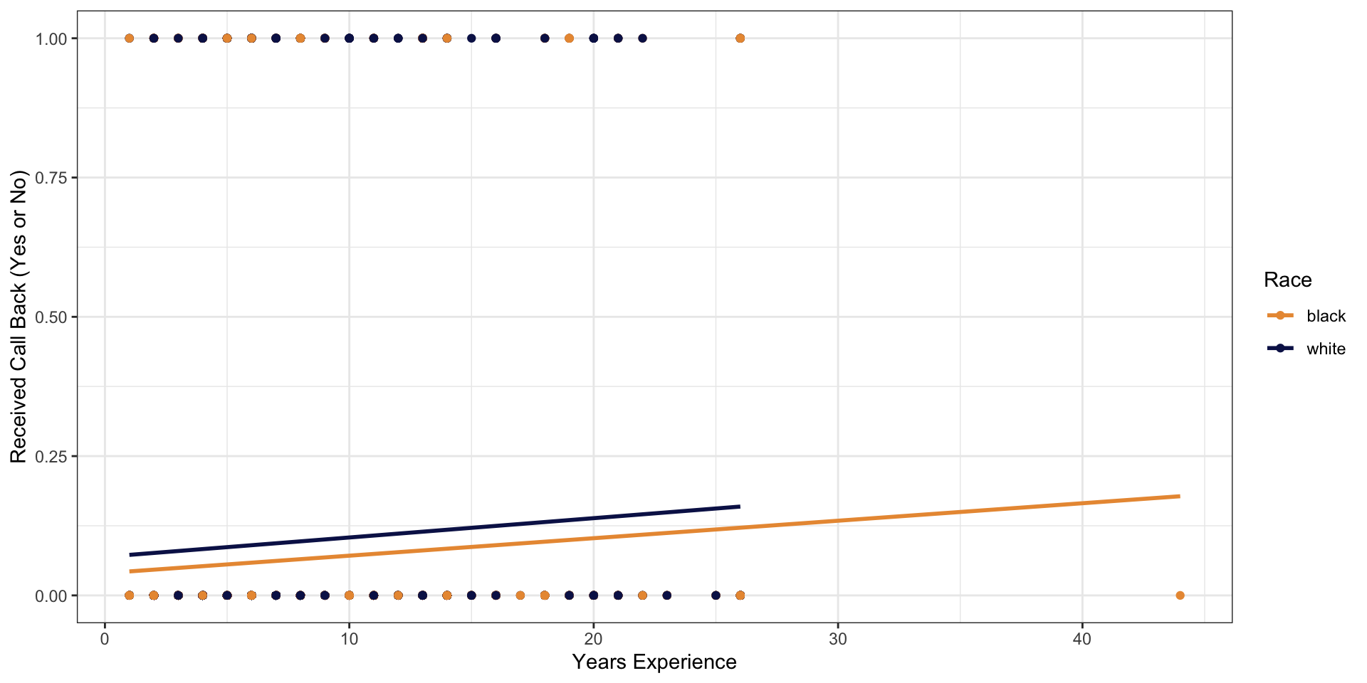
Logit function
Logit function
The logit function takes a value between 0 and 1 and maps it to a value between \(-\infty\) and \(\infty\)
Inverse logit (logistic) function:
\[g^{-1}(x) = \frac{\exp(x)}{1+\exp(x)} = \frac{1}{1+\exp(-x)}\]
- The inverse logit function takes a value between \(-\infty\) and \(\infty\) and maps it to a value between 0 and 1
Logistic regression model
- \(y_i \sim \text{Bern}(p_i)\)
- \(\eta_i = \beta_0+ \beta_1 x_{1,i} + \cdots + \beta_n x_{n,i}\)
- \(\text{logit}(p_i) = \eta_i\)
Logistic regression model
\(\text{logit}(p_i) = \eta_i = \beta_0+ \beta_1 x_{1,i} + \cdots + \beta_n x_{n,i}\)
Now take inverse logit to get \(p\)
\[p_i = \frac{\exp(\beta_0+\beta_1 x_{1,i} + \cdots + \beta_k x_{k,i})}{1+\exp(\beta_0+\beta_1 x_{1,i} + \cdots + \beta_k x_{k,i})}\]
Running logistic regression
Implementation is not very difficult now that we know how to run a linear model
We just need to update our code to run a GLM
- specify the model with
logistic_reg() - use
"glm"instead of"lm"as the engine
- define
family = "binomial"for the link function to be used in the model
- specify the model with
Running logistic regression
discrim_fit <- logistic_reg() %>%
  set_engine("glm") %>%
  fit(factor(received_callback) ~ years_experience, data = resume, family = "binomial")
tidy(discrim_fit)
# A tibble: 2 × 5
term estimate std.error statistic p.value
<chr> <dbl> <dbl> <dbl> <dbl>
1 (Intercept) -2.76 0.0962 -28.7 5.58e-181
2 years_experience 0.0391 0.00918 4.26 2.07e- 5Interpretation
The results here are for the linear model predicting \(\eta_i\)
This makes them hard to interpret
We need to convert into predicted probabilities
- We can use the inverse logit function to do this
Interpretation
The intercept is -2.76
When all predictors at 0, \(\eta_i = -2.76\)
Logistic function: \(\frac{exp(\eta_i)}{( 1 + exp(\eta_i))}\)
Predicted Probabilities
Predicted Probabilities
y_hat <- predict(discrim_fit, newdata, type = "raw")

# Use inverse logit function to get predicted probabilities
p_hat <- exp(y_hat) / (1 + exp(y_hat))

# merge to our new data
newdata <- newdata %>%
  bind_cols(
    y_hat = y_hat,
    p_hat = p_hat
  )
newdata
# A tibble: 4 × 3
years_experience y_hat p_hat
<dbl> <dbl> <dbl>
1 0 -2.76 0.0595
2 5 -2.56 0.0715
3 15 -2.17 0.102
4 25 -1.78 0.144 Predicted Probabilities
expand for full code
ggplot(newdata, aes(y=p_hat, x = years_experience)) +
  geom_point(color = "#0C1956") +
  geom_line(color = "#0C1956") +
  scale_x_continuous(breaks=seq(0, 30, 5)) +
  scale_y_continuous(breaks=seq(0, .75, .05)) +
  ylim(0, .25) +
  labs(
    x = "Years Experience",
    y = "Predicted Probability of Call Back",
    title = ""
  ) +
  theme_bw()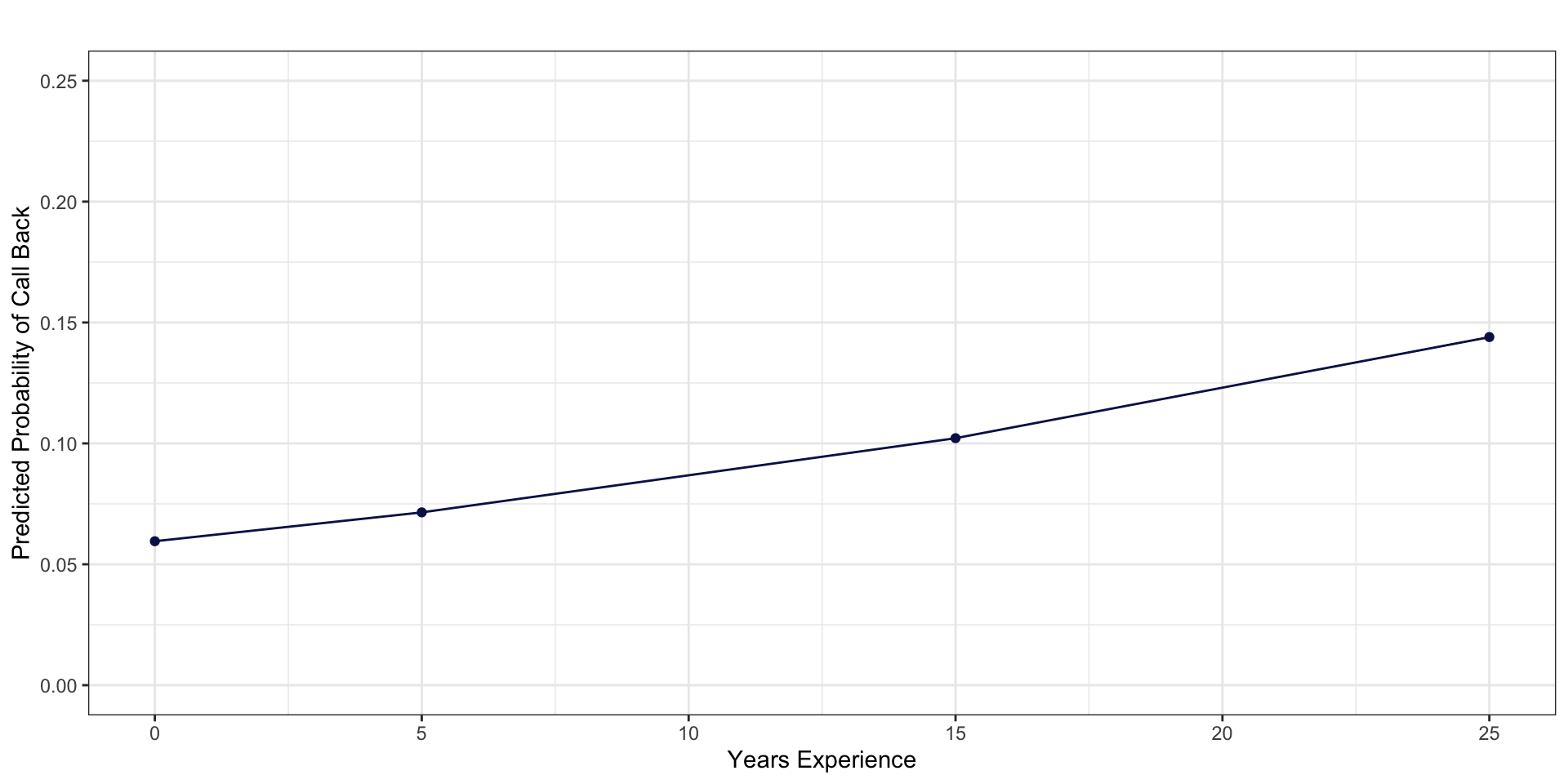
Racial Discrimination Model
discrim_fit <- logistic_reg() %>%
  set_engine("glm") %>%
  fit(factor(received_callback) ~ race, data = resume, family = "binomial")
tidy(discrim_fit)
# A tibble: 2 × 5
term estimate std.error statistic p.value
<chr> <dbl> <dbl> <dbl> <dbl>
1 (Intercept) -2.67 0.0825 -32.4 1.59e-230
2 racewhite 0.438 0.107 4.08 4.45e- 5Predicted Probabilities
Predicted Probabilities
y_hat <- predict(discrim_fit, newdata, type = "raw")

# Take inverse logit of y_hat to get predicted probabilities
p_hat <- exp(y_hat) / (1 + exp(y_hat))

# merge to our new data
newdata <- newdata %>%
  bind_cols(
    y_hat = y_hat,
    p_hat = p_hat
  )
newdata
# A tibble: 2 × 3
race y_hat p_hat
<chr> <dbl> <dbl>
1 white -2.24 0.0965
2 black -2.67 0.0645Is this difference due to chance?
Is this difference due to chance?
Very unlikely to be due to chance
Multiple Predictors
discrim_fit <- logistic_reg() %>%
  set_engine("glm") %>%
  fit(factor(received_callback) ~ race + years_experience, data = resume, family = "binomial")
tidy(discrim_fit)
# A tibble: 3 × 5
term estimate std.error statistic p.value
<chr> <dbl> <dbl> <dbl> <dbl>
1 (Intercept) -3.00 0.116 -25.9 2.37e-148
2 racewhite 0.438 0.108 4.08 4.56e- 5
3 years_experience 0.0391 0.00920 4.25 2.14e- 5Predicted Probabilities
# variable names need to be same as in dataset
newdata <- tibble(
  race = c("white", "black", "white", "black", "white", "black", "white", "black"),
  years_experience = c(0, 0, 10, 10, 20, 20, 30, 30)
  )
newdata
# A tibble: 8 × 2
race years_experience
<chr> <dbl>
1 white 0
2 black 0
3 white 10
4 black 10
5 white 20
6 black 20
7 white 30
8 black 30Predicted Probabilities
y_hat <- predict(discrim_fit, newdata, type = "raw")
p_hat <- exp(y_hat) / (1 + exp(y_hat))
# merge to our new data
newdata <- newdata %>%
bind_cols(
y_hat = y_hat,
p_hat = p_hat
)
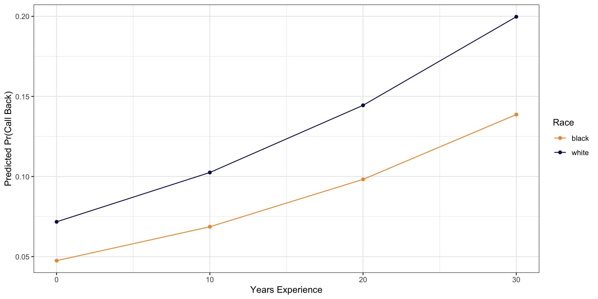
newdata# A tibble: 8 × 4
race years_experience y_hat p_hat
<chr> <dbl> <dbl> <dbl>
1 white 0 -2.56 0.0717
2 black 0 -3.00 0.0475
3 white 10 -2.17 0.103
4 black 10 -2.61 0.0686
5 white 20 -1.78 0.144
6 black 20 -2.22 0.0982
7 white 30 -1.39 0.200
8 black 30 -1.83 0.139 Plotting Predicted Probabilities
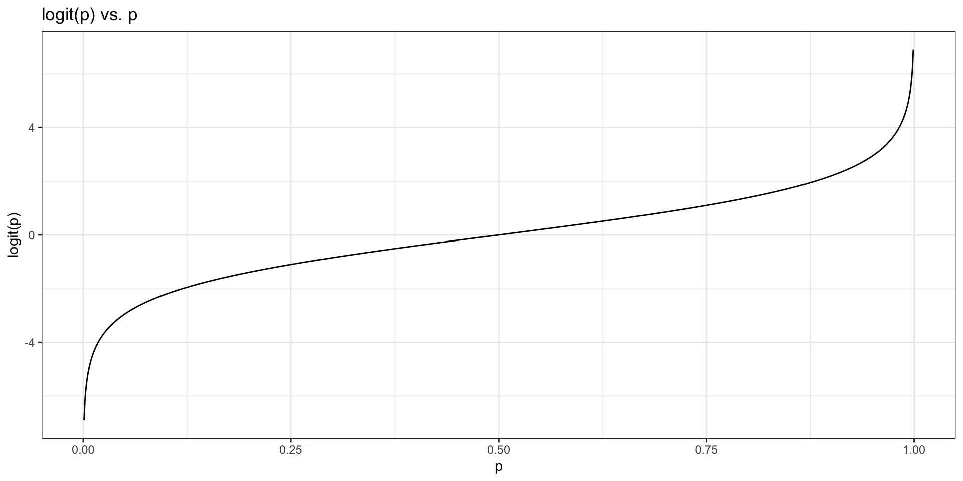
Plotting Predicted Probabilities
In a linear model with no interactions, the impact of race would not vary depending on other values of other measures (years_experience).
This is not the case for logistic regression because of the transformation.
For interpretation, it is important to set the values of the other predictors
Your Turn: Fit and Interpret Logistic Regression
 [1] "spam"         "to_multiple"  "from"         "cc"           "sent_email"
 [6] "time"         "image"        "attach"       "dollar"       "winner"
[11] "inherit"      "viagra"       "password"     "num_char"     "line_breaks"
[16] "format"       "re_subj"      "exclaim_subj" "urgent_subj"  "exclaim_mess"
[21] "number"
  no  yes
3857   64
Spam Filter: Fit Model
Spam Filter: Data for prediction
Spam Filter: Predicted Probabilities
Try a different variable
 [1] "spam"         "to_multiple"  "from"         "cc"           "sent_email"
 [6] "time"         "image"        "attach"       "dollar"       "winner"
[11] "inherit"      "viagra"       "password"     "num_char"     "line_breaks"
[16] "format"       "re_subj"      "exclaim_subj" "urgent_subj"  "exclaim_mess"
[21] "number"
   0    1
3914    7
Use
table(email$VARNAME)to determine values of the variable you choose.Run logistic regresson model and generate predicted probabilities of being spam for each value of the variable
Run model with two predictors: winner and the variable you choose. Calculate predicted probabilities.
Bonus: Run interaction model and calculate predicted probabilities.