# Load countrycode
library(countrycode)

# Create new iso3c variable
democracy <- democracy |>
  mutate(iso3c = countrycode(sourcevar = vdem_ctry_id, # what we are converting
        origin = "vdem",         # we are converting from vdem
        destination = "wb"))  |> # and converting to the WB iso3c code
  relocate(iso3c, .after = vdem_ctry_id) # move iso3c

# View the data
glimpse(democracy)Merging and Summarizing Data
May 19, 2025
Merging Data
Merging Data Frames
- Often we have data from two different sources
- Results in two data frames
- How to make them one so we can analyze?
- Key questions
- What is the unit of analysis?
- What is/are the corresponding identifier variables?
- Are the identifier variables in common?
- Or do they have to be added/transformed to match?
Merging WB and V-Dem Data
- These are both time-series, country-level data
- Need to merge by country-year
- Year is easy
- But there are many different country codes
- Can use
countrycodepackage to assign country codes
countrycode Example
Try it Yourself
- Using your democracy data frame from the last lesson
- Use
mutate()andcountrycode()to add iso3c country codes - Use
relocateto move your iso3c code to the “front” of your data frame (optional)
Types of Joins in dplyr
- Mutating versus filtering joins
- Four types of mutating joins
inner_join()full_join()left_join()right_join()
- For the most part we will use
left_join()
left_join() Example
# Load readr
library(readr)

# Perform left join using common iso3c variable and year
dem_women <- left_join(democracy, women_emp, by = c("iso3c", "year")) |>
  rename(country = country.x) |> # rename country.x
  select(!country.y)             # crop country.y

# Save as .csv for future use
write_csv(dem_women, "data/dem_women.csv")

# View the data
glimpse(dem_women)
Try it Yourself
- Take your V-Dem data frame and your World Bank data frame
- Using
left_join()to merge on country code and year - Along the way, use
rename()andselect()to insure you have just one country name
Group, Summarize and Arrange
Group, Summarize and Arrange
group_by(),summarize(),arrange()- A very common sequence of
dplyrverbs:- Take an average or some other statistic for a group
- Rank from high to low values of summary value
Example: Take Averages by Region
# group_by(), summarize() and arrange()
dem_region <- democracy |> # save result as new object
  group_by(region)  |> # group data by region
  summarize(           # summarize following vars (by region)
    polyarchy = mean(polyarchy, na.rm = TRUE), # calculate mean, remove NAs
    gdp_pc = mean(gdp_pc, na.rm = TRUE)
  ) |>
  arrange(desc(polyarchy)) # arrange in descending order by polyarchy score

# Save as .csv for future use
write_csv(dem_region, "data/dem_summary.csv")

# View the data
glimpse(dem_summary)
Use group_by() to group all data across countries and years by region…
# group_by(), summarize() and arrange()
dem_region <- democracy |> # save result as new object
  group_by(region)  |> # group data by region
  summarize(           # summarize following vars (by region)
    polyarchy = mean(polyarchy, na.rm = TRUE), # calculate mean, remove NAs
    gdp_pc = mean(gdp_pc, na.rm = TRUE)
  ) |>
  arrange(desc(polyarchy)) # arrange in descending order by polyarchy score

# Save as .csv for future use
write_csv(dem_region, "data/dem_summary.csv")

# View the data
glimpse(dem_summary)
Use summarize() to get the regional means polyarchy and gpd_pc….
# group_by(), summarize() and arrange()
dem_region <- democracy |> # save result as new object
  group_by(region)  |> # group data by region
  summarize(           # summarize following vars (by region)
    polyarchy = mean(polyarchy, na.rm = TRUE), # calculate mean, remove NAs
    gdp_pc = mean(gdp_pc, na.rm = TRUE)
  ) |>
  arrange(desc(polyarchy)) # arrange in descending order by polyarchy score

# Save as .csv for future use
write_csv(dem_region, "data/dem_summary.csv")

# View the data
glimpse(dem_summary)
Then use arrange() with desc() to sort in descending order by polyarchy score…
# group_by(), summarize() and arrange()
dem_region <- democracy |> # save result as new object
  group_by(region)  |> # group data by region
  summarize(           # summarize following vars (by region)
    polyarchy = mean(polyarchy, na.rm = TRUE), # calculate mean, remove NAs
    gdp_pc = mean(gdp_pc, na.rm = TRUE)
  ) |>
  arrange(desc(polyarchy)) # arrange in descending order by polyarchy score

# Save as .csv for future use
write_csv(dem_region, "data/dem_summary.csv")

# View the data
glimpse(dem_summary)
Try it Yourself
- Try running a
group_by(),summarize()andarrange()in your Quarto document - Try changing the parameters to answer these questions:
- Try summarizing the data with a different function for one or more of the variables.
- What is the median value of
polyarchyfor The West? - What is the max value of
gdp_pcfor Eastern Europe? - What is the standard deviation of
flfpfor Africa? - What is the interquartile range of
women_repfor the Middle East?
- Now try grouping by country instead of region.
- What is the median value of
polyarchyfor Sweden? - What is the max value of
gdp_pcNew Zealand? - What is the standard deviation of
flfpfor Spain? - What is the interquartile range of
women_repfor Germany?
Sort countries in descending order based on the mean value of
gdp_pc(instead of the median value ofpolyarchy). Which country ranks first based on this sorting?Now try sorting countries in ascending order based on the median value of
women_rep(hint: delete “desc” from thearrange()call). Which country ranks at the “top” of the list?
05:00
Choropleth Maps
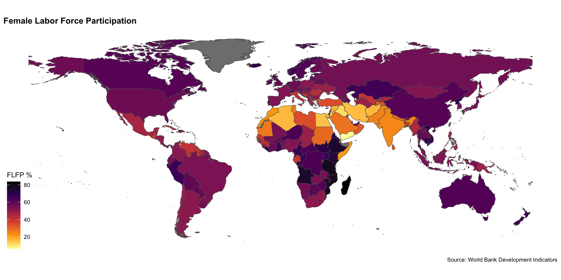
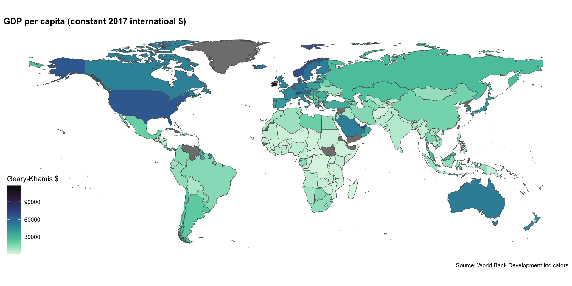
Choropleth Maps
- Choropleth maps are shaded maps that show variation in a variable across geographic space
- Now that you have a handle on how to merge data, you should be able to make one!
Choropleth Map
Choropleth Map
The rnaturalearth package
rnaturalearthis a package that provides access to shapefiles for countries, states, and provinces- Uses the Natural Earth dataset which features the “natural earth” projection
- Contrasts with Mercator projection used by Google Maps, etc.
- Also uses simple features (sf) dataframes
- A new way of storing spatial data in R
- Allows for easy storage, manipulation and plotting
Mercator Projection
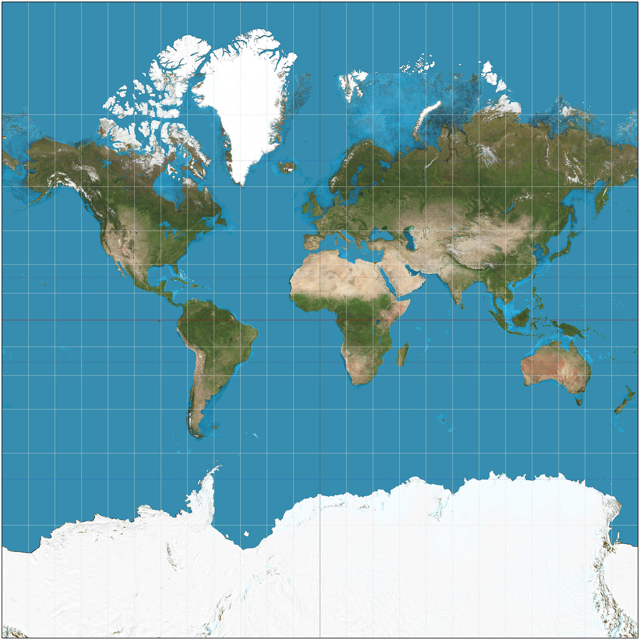
Source: Wikipedia
Natural Earth Projection
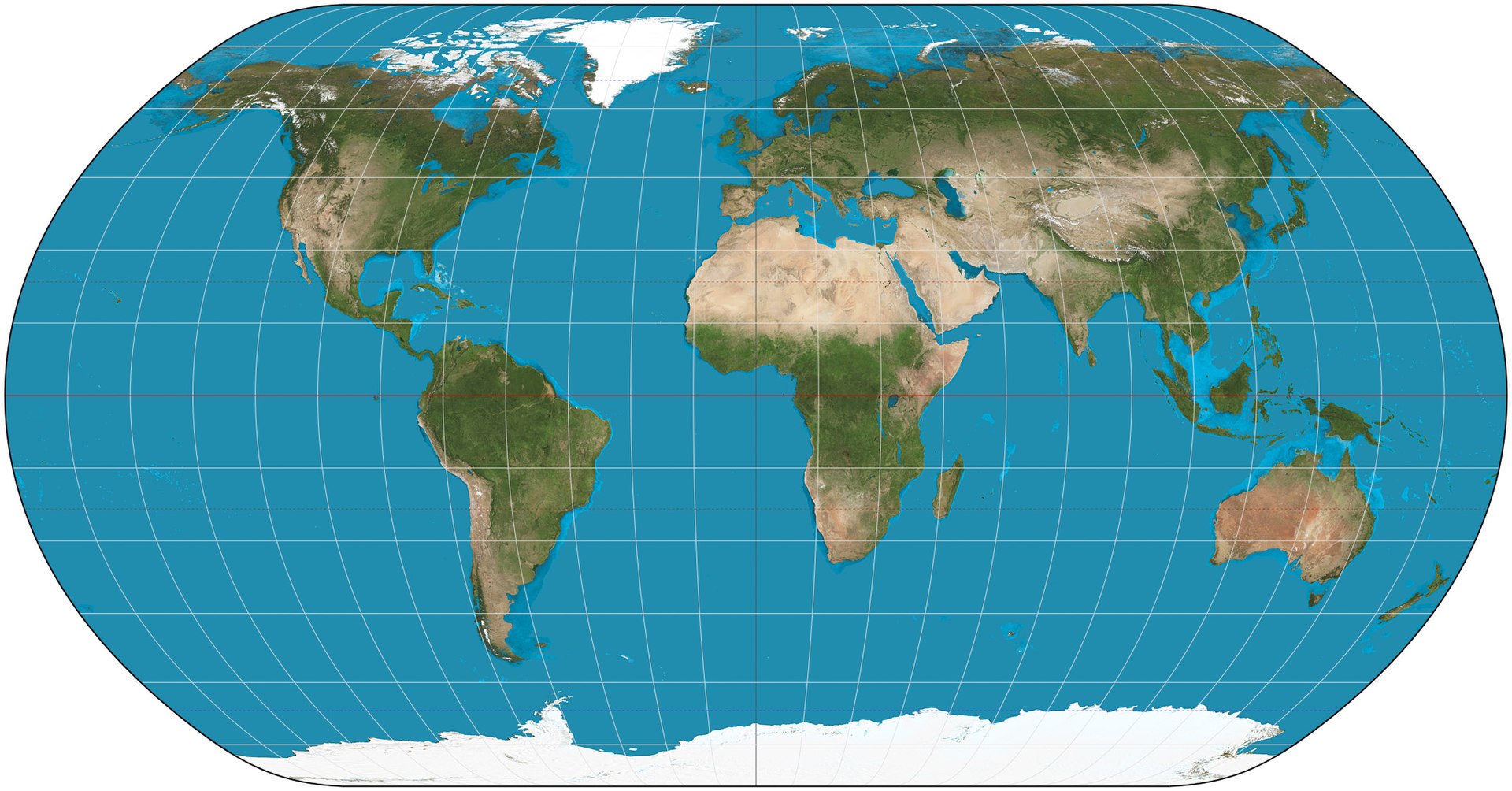
Source: Wikipedia
Simple Features
Map Code
Grab country shapes with ne_countries()
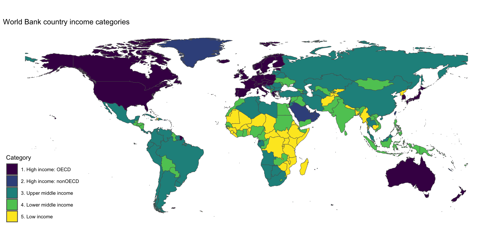
Basic Choropleth Map
Make a map using geom_sf() from ggplot2.
That gives us…
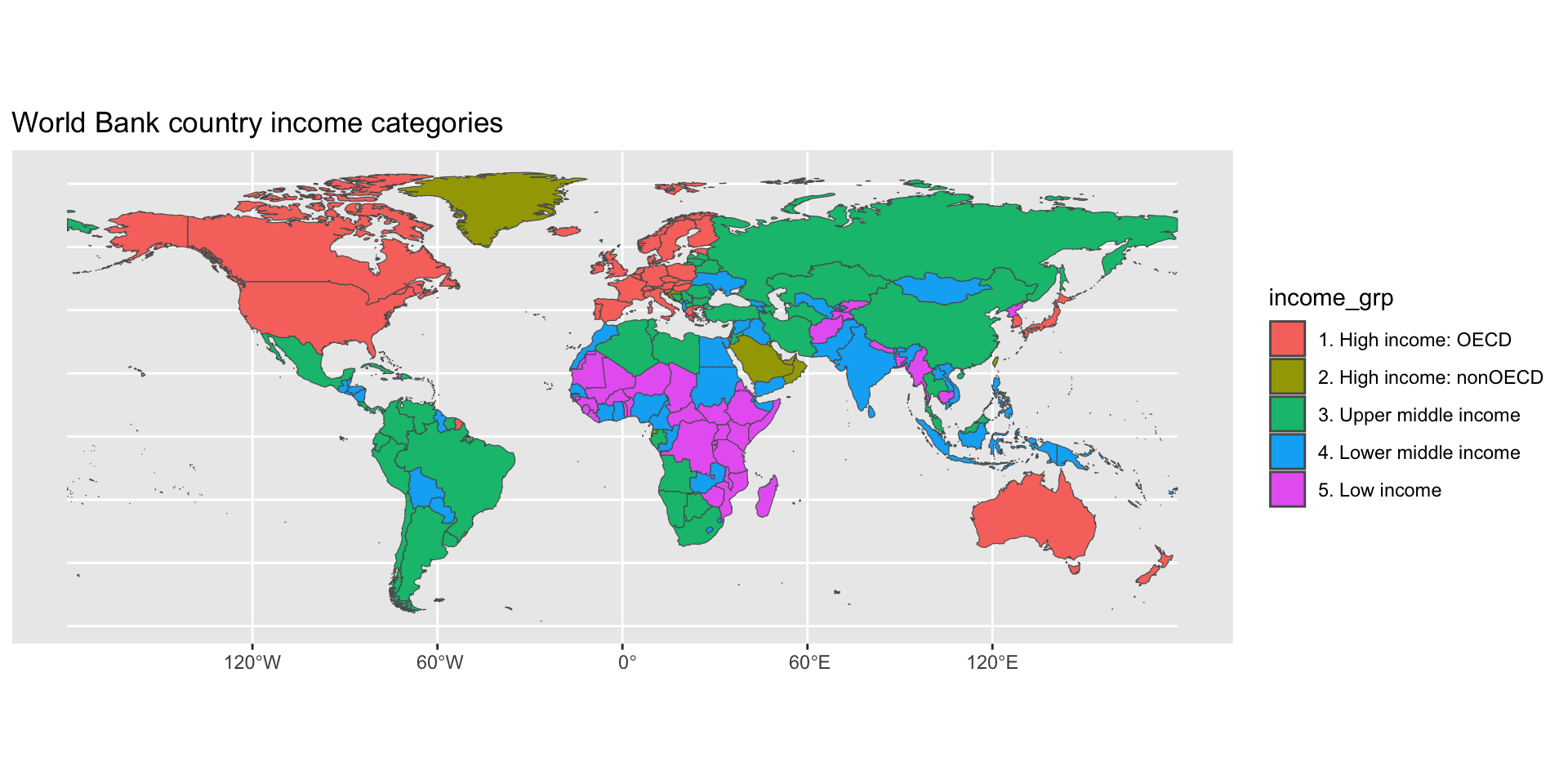
Beautiful Map
Change label of legend with fill=, add viridis color scheme and change theme with theme_map() from ggthemes.
And now we have…
Your Turn!
- Make a map of WB income categories
- Grab country shapes and store data in an object
- Use
geom_sf()to make the map - Style the map with
labs()andscale_fill_viridis_d() - Try mapping a different variable (check on this)
05:00
Map Other Data
Map Other Data
Grab data from the WB, join with country shapes…
# Load wbstats
library(wbstats)
# Grab oil rents data
oil_rents_df <- wb_data(c(oil_rents_gdp = "NY.GDP.PETR.RT.ZS"), mrnev = 1)
# Join with country shapes
rents_map_df <- left_join(world_map_df, oil_rents_df, join_by(iso_a3 == iso3c))
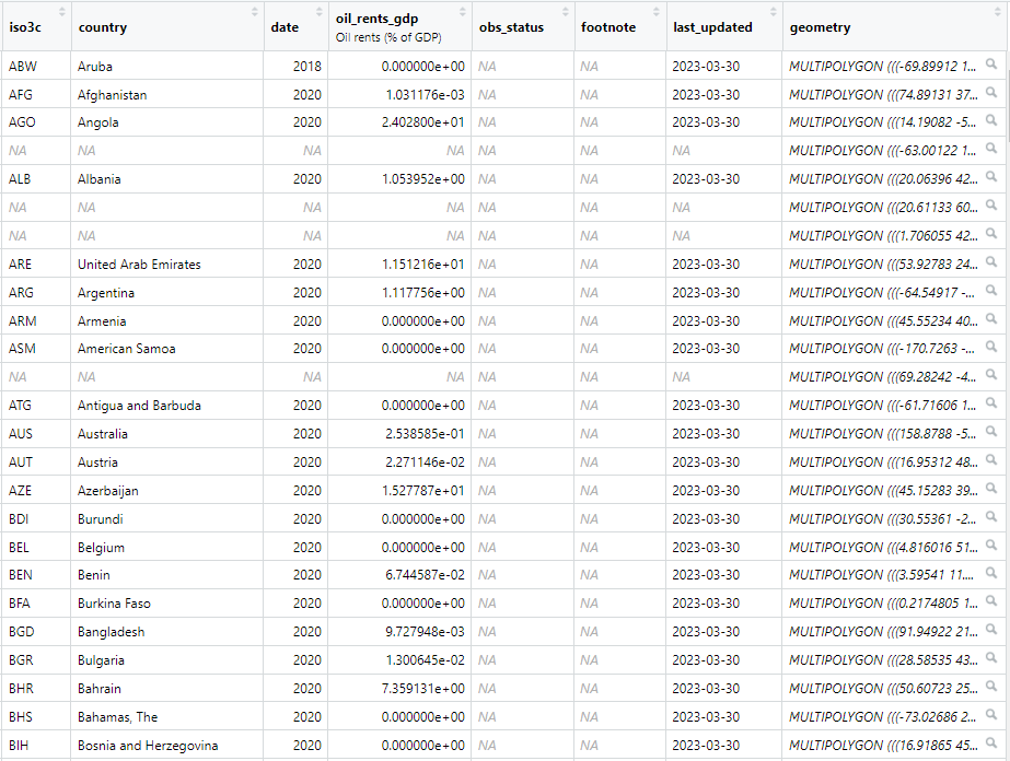
# Have a look at the special features column
rents_map_df |>
select(last_col(5):last_col()) |> #select last 5 columns of df
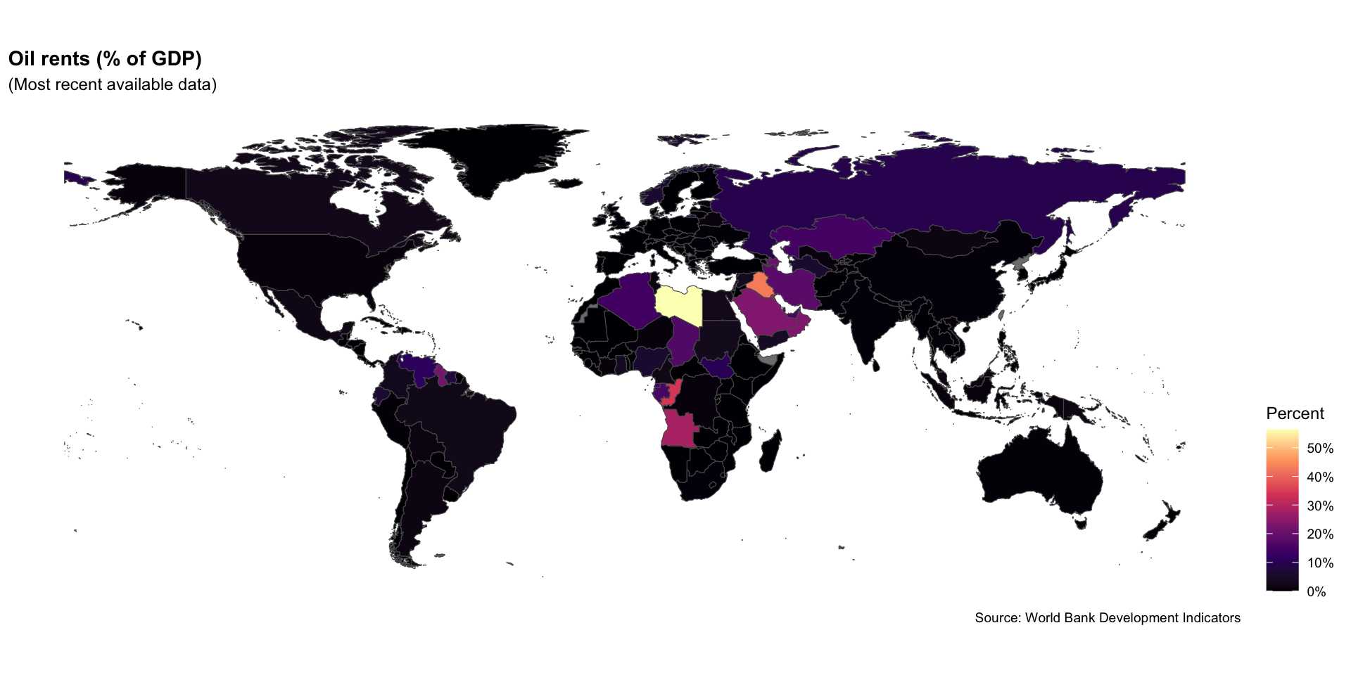
glimpse()Map Other Data
ggplot(data = rents_map_df) +
  geom_sf(aes(fill = oil_rents_gdp)) + # shade based on oil rents
  labs(
    title = "Oil rents (% of GDP)",
    subtitle = "(Most recent available data)", # add subtitle
    fill = "Percent",
    caption = "Source: World Bank Development Indicators"
    ) +
  theme_map() +
  theme(
    legend.position = "right",
    plot.title = element_text(face = "bold"), # move legend
    ) +
  scale_fill_viridis_c( # chg from discrete (_d) to continuous (_c)
      option = "magma", #  chg to magma theme
      labels = scales::label_percent(scale = 1) # add % label for legend
      )
Your Turn!
- Try mapping a favorite variable from the World Bank
- First, download the relevant data using
wbstats - Then merge it with your country shapes
- Map using
geom_sf() - Beautify your map!
05:00
Map Some V-Dem Data
- Now try mapping some V-Dem data
- Remind yourself of how to download data from V-Dem
- You will have to convert country codes to iso3c
- Then merge with country shapes
- Then map your V-Dem indicator!
05:00