IAFF 6501 – Inference, Sampling, and Study Design

Inference

Prior classes focused on data visualization and summary
Now, we turn to inference: the kinds of conclusions we can and want to draw from our data

Target Population

In data analysis, we are usually interested in saying something about a Target Population.

What proportion of adult Russians support the war in Ukraine?
- Target population: adult Russians (age 18+)
How many US college students check social media during their classes?
- Target population: US college students

Sample

In many instances, we have a Sample

We cannot talk to every Russian
We cannot talk to all college students

Parameters vs Statistics

The Parameter: this is the value of a calculation for the entire target population
The Statistic: this is what we calculate on our sample
- We calculate a statistic in order to say something about the parameter

Inference

Inference is the act of “making a guess” about some unknown.
Statistical inference: making a good guess about a population from a sample
Causal inference: did X cause Y? [topic for later classes]

Let’s Move to an IA Example

Hypothetical

Question: What proportion of adult (18+) Russian citizens support the war in Ukraine?
What is the Population of interest?
What is the Parameter of interest?

Russia Hypothetical

Our population has 4000 supporters, and 6000 non-supporters
What is the population parameter?

Russia Example

This is the Population: in real research, we do not have this information!

pop <- c(rep(1, 4000), rep(0, 6000))
pop <- as_tibble(pop)
table(pop)

value
   0    1 
6000 4000

mean(pop$value)

[1] 0.4

Let’s take a random sample of 20

s1 <- slice_sample(pop, n= 20)
glimpse(s1)

Rows: 20
Columns: 1
$ value <dbl> 0, 0, 0, 0, 1, 0, 0, 0, 1, 1, 0, 1, 0, 0, 0, 0, 0, 1, 0, 0

mean(s1$value)

[1] 0.25

Our random sample of 20

What does it mean to say that this is a random sample?

Our random sample of 20

What does it mean to say that this is a random sample?
All units in the population have an equal Probability of being selected

Our random sample of 20

When I calculate the mean in the sample, what am I calculating?

Our random sample of 20

When I calculate the mean in the sample, what am I calculating?
Our Estimate of the population parameter

Let’s take another random sample of 20

s2 <- slice_sample(pop, n= 20)
mean(s2$value)

[1] 0.45

Let’s take another….

s3 <- slice_sample(pop, n= 20)
mean(s3$value)

[1] 0.5

Let’s do this 1,000 more times

# Gather 1,000 estimates
sims <- 1000
# Store the sample means in this object called "ests"
ests <- rep(NA, sims)
# For loops allow us to run the same procedure many times
for(i in 1:sims){
  sample <- slice_sample(pop, n= 20)
    # store mean in our vector of estimates
    ests[i] <- mean(sample$value)
}
ests <- as_tibble(ests)

What is stored in this vector?

ests

# A tibble: 1,000 × 1
   value
   <dbl>
 1  0.6 
 2  0.5 
 3  0.6 
 4  0.35
 5  0.3 
 6  0.45
 7  0.55
 8  0.55
 9  0.4 
10  0.35
# ℹ 990 more rows

Where should the distribution of this set of estimates be centered?

Or, what should the mean of ests be?

Where should the distribution of this set of estimates be centered?

mean <- mean(ests$value)
mean

[1] 0.39315

Distribution of estimates

Bias

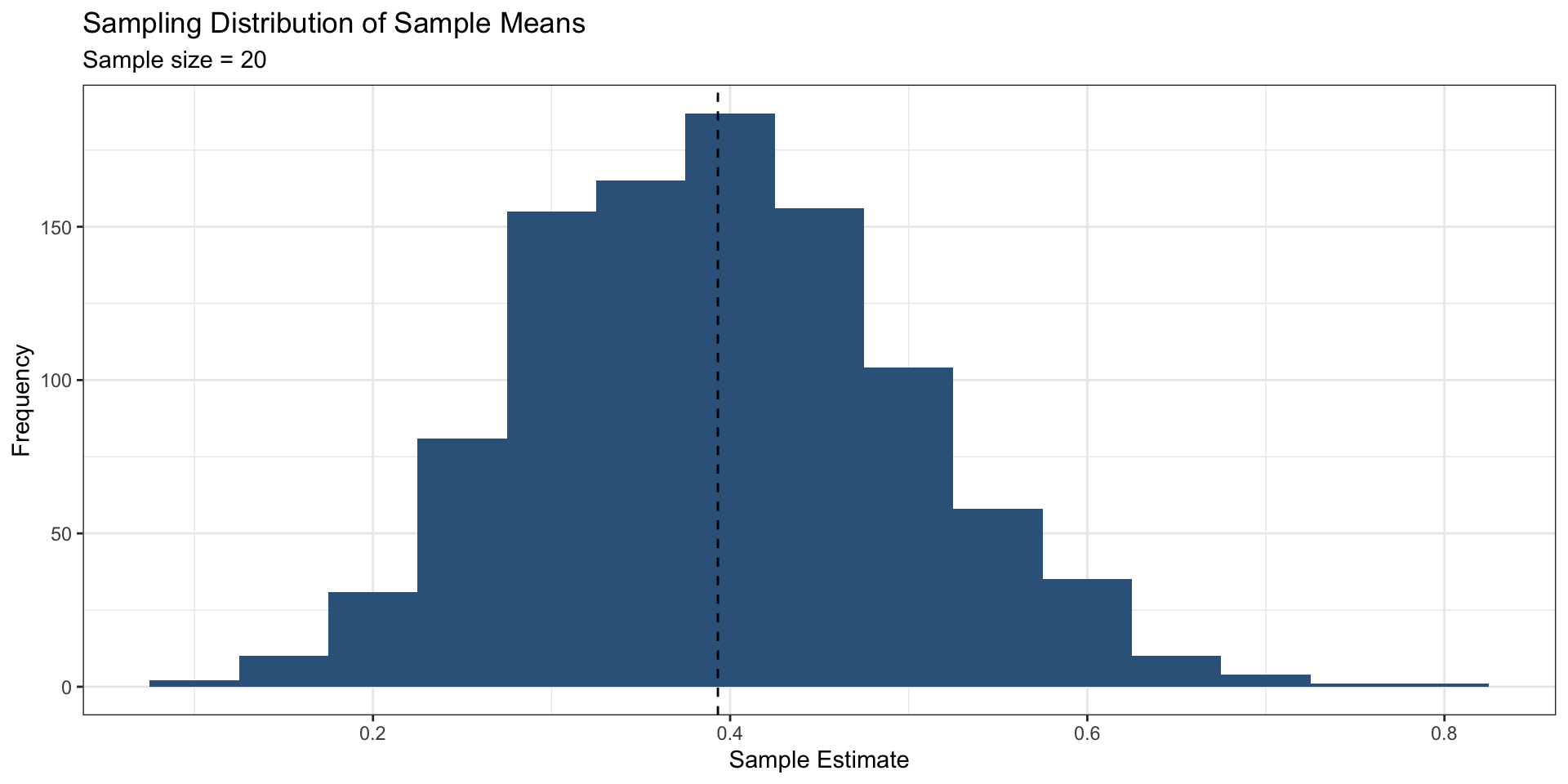
The mean of ests is almost exactly the same as the population mean (which we know because we set it)
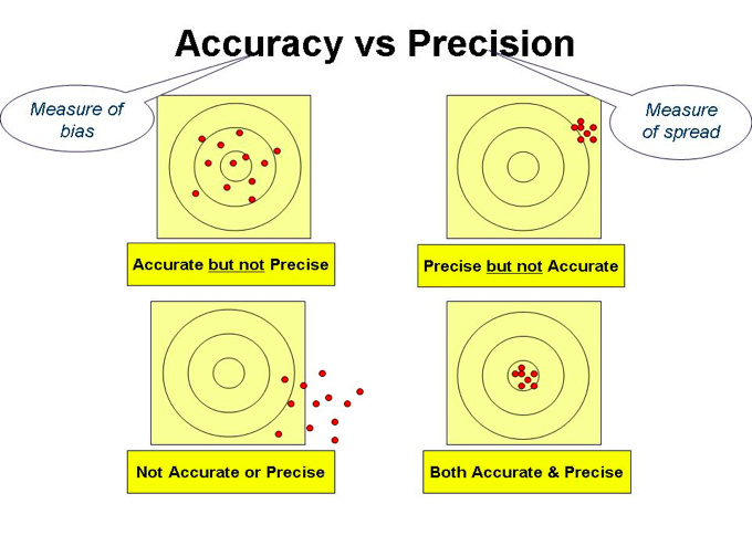
This means that our procedure (random sampling + taking the mean) for estimating the population mean is unbiased
- on average, we get the “right” answer

Bias

Will unbiased procedures get the “right” answer every time?

Sampling Variability

An unbiased procedure does not guarantee that we will get the “right” answer every time
This is due to random chance, or sampling variability

Sampling Distribution (n = 20)

Standard Error

Standard deviation of the sampling distribution
Characterizes the spread of the sampling distribution

sd(ests$value)

[1] 0.1058148

Sample size and Sampling Variability

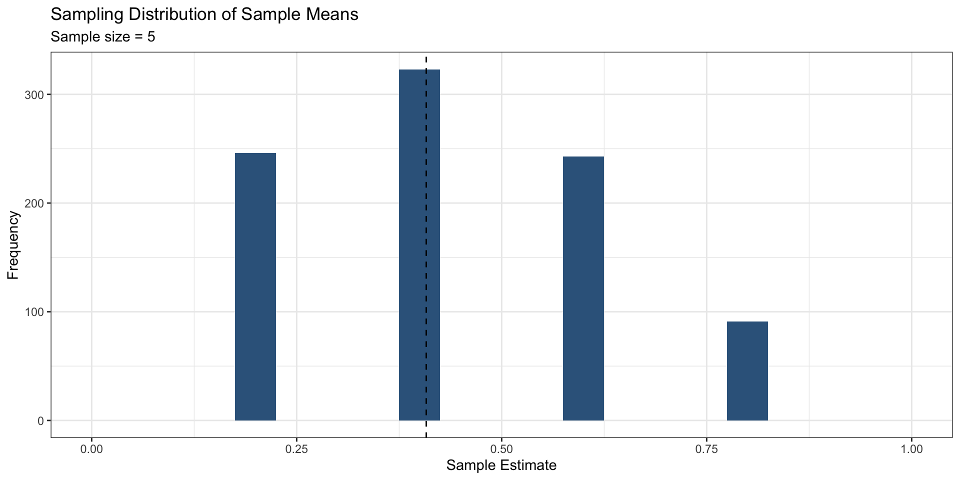
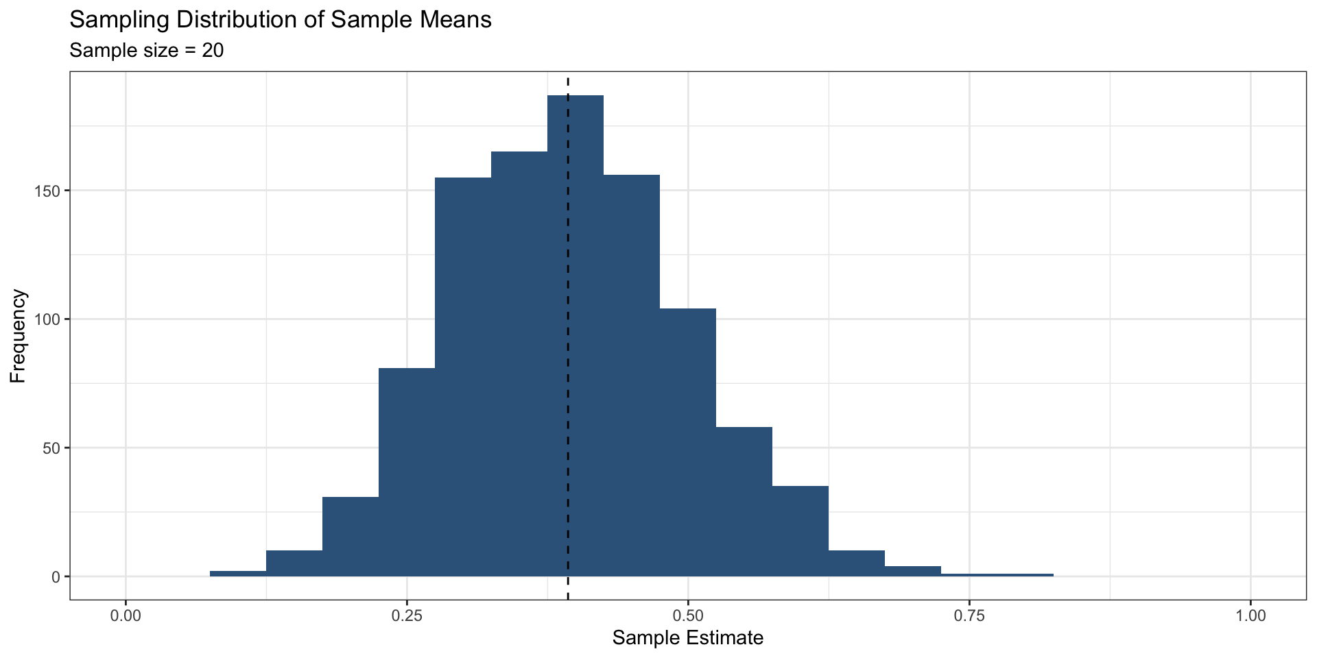
Repeat the simulations conducted above:
- Once with n = 5
- Once with n = 20
- Once with n = 200
For each: Are these biased or unbiased procedures?
Visualize the sampling distributions using a histogram: how are they different?
Calculate the standard errors: how are they different?
Discuss with partner: Why are the sampling distributions and standard errors different?

Let’s try N=5

# RUn 1000 simulations
sims <- 1000
# Store the sample means in this
ests5 <- rep(NA, sims)
# For loops allow us to run the same procedure many times
for(i in 1:sims){
  sample <- slice_sample(pop, n = 5)
    ests5[i] <- mean(sample$value)
  }    
ests5 <- as_tibble(ests5)

Let’s try N=200

sims <- 1000
# Store the sample means in this
ests200 <- rep(NA, sims)
# For loops allow us to run the same procedure many times
for(i in 1:sims){
  sample <- slice_sample(pop, n= 200)
    ests200[i] <- mean(sample$value)
}  
ests200 <- as_tibble(ests200)

Sampling Distribution, Sample Size = 5

Sampling Distribution, Sample Size = 20

Sampling Distribution, Sample Size = 200

Compare Standard errors

# N = 5
sd(ests5$value)

[1] 0.2276573

# N = 20
sd(ests$value)

[1] 0.1058148

#N = 200
sd(ests200$value)

[1] 0.03511064

Why does changing sample size matter?

Central Limit Theorem

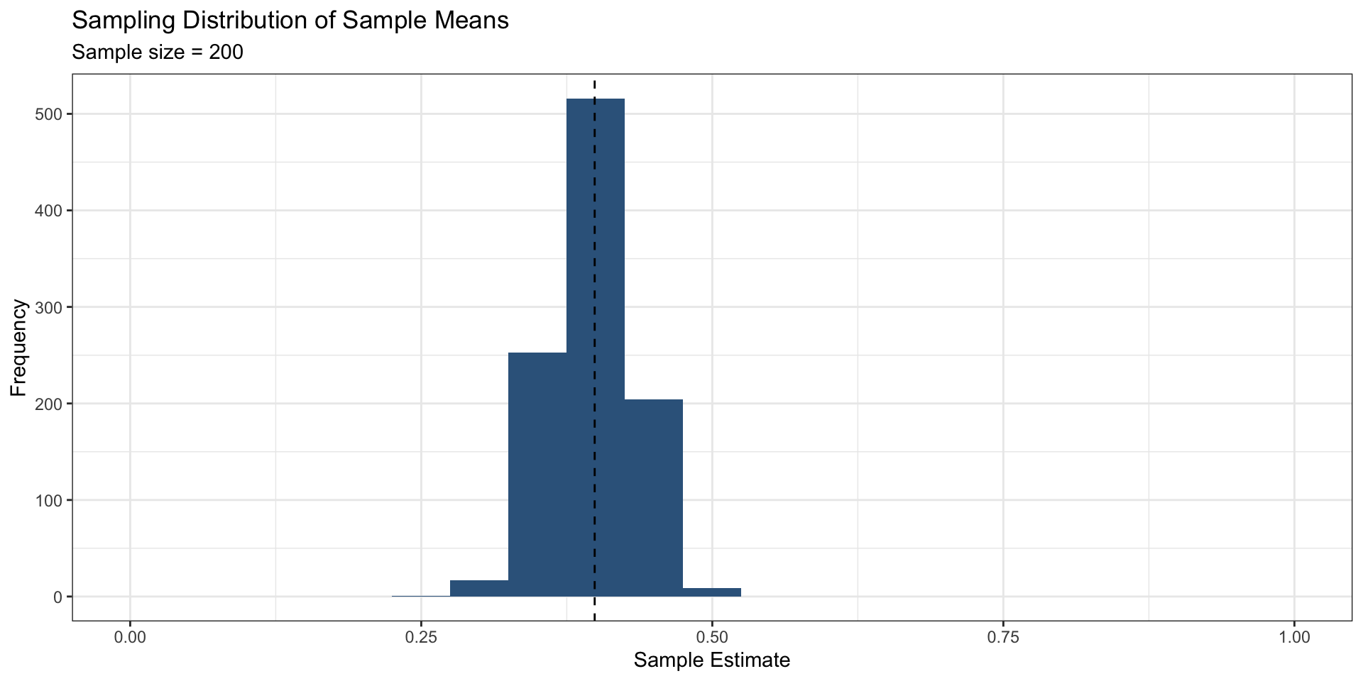
As sample size gets bigger . . .

The spread of the sampling distribution gets narrower
The shape of the sampling distributions becomes more normally distributed
- Important for mathematical calculations in statistics (not big focus for us)

Bias vs Precision

A procedure is unbiased if it generates the “right” answer, on average

Precision refers to variability: procedures with less sampling variability will be more precise
- all else equal, a greater sample size will increase precision

Why did we do these simulations?

They provide a foundation for statistical inference and for characterizing uncertainty in our estimates, our next topic

The best research designs will try to maximize or achieve good balance on bias vs precision

Research Design Implications

Questions?

Research Design Scenarios

Discuss with partner

Scenario 1

A development organization is trying to build evidence demonstrating the impact of their programming on political participation. The program has hundreds of participants. Five program participants volunteered to provide information on their political participation and each reports that they participate much more after they were in the program. The development organization concludes that the program had the intended impact of increasing political participation.

Using language from earlier in class, critically assess this conclusion.

Scenario 1A

A development organization is trying to build evidence demonstrating the impact of their programming on political participation. The program has hundreds of participants. Five program participants were randomly selected to provide information on their political participation and each reports that they participate much more after they were in the program. The development organization concludes that the program had the intended impact of increasing political participation.

Using language from earlier in class, critically assess this research design and conclusion.

Scenario 2

A polling firm is trying to estimate the proportion of likely voters that will vote for President Biden. They draw a random sample of 1000 adult Americans and ask them whether they intend to vote for Biden. From this, they calculate the proportion who intend to vote for Biden.

What is the target population?
What is the statistic (or estimate)?
Is this estimate a good guess of the population parameter?

Scenario 3

In 2016, polling firms using random sampling tried to estimate the proportion of adult Americans who would vote for Trump. In surveys in America, the response rate is very low (~10 percent) and people without a college education are less likely to respond to surveys than are other Americans.

What is the target population?
One firm claims despite the low response rate their procedure is unbiased because of random sampling: based on the information above, do you agree?

Scenario 4

Researchers are interested in studying the political attitudes of ex-combatants in a civil war. They have a limited budget and are debating the best research design. In option A, they use random sampling, which is very expensive given the target population (they have to enumerate ex-combatants and then track them down, which is resource intensive). This would allow them to survey 20 ex-combatants given the budget. In option B, they use snowball sampling, where ex-combatants introduce the researchers to other ex-combatants that they know. This is much cheaper, and would result in a sample size of 250.

What are the costs and benfits of option A?
What are the costs and benefits of option B?
Imagine the researchers are able to make reasonably good guesses about how much bias would be generated by snowball sampling: when would option B be a better choice? when would option A be better?

Bias-Variance Tradeoff

Sometimes, a little bit of bias is OK, if it buys us a lot more precision [small bias + high precision]
An unbiased study with very low precision is not informative (as we will discover more in future classes)
But this depends on how much bias there is: high bias + high precision is not a good outcome.