Hypothesis Testing 2

Associations between Variables

January 29, 2025

Relationships Between Variables


Simple example: does treatment have an impact on y?

Or, is there an association between these two variables

Hypothetical Data

library(tidyverse)
myData <- tibble(
  treatment = c(1, 0, 0, 0, 0, 0, 1),
  y = c(15, 15, 20, 20, 10, 15, 30)
) %>% 
  mutate(treatment = factor(treatment))

Hypothetical Data

head(myData, n = 7)
# A tibble: 7 × 2
  treatment     y
  <fct>     <dbl>
1 1            15
2 0            15
3 0            20
4 0            20
5 0            10
6 0            15
7 1            30

We can calculate the means in each treatment group

mns <- myData %>% 
  group_by(treatment) %>% 
  summarise(means = mean(y))
mns
# A tibble: 2 × 2
  treatment means
  <fct>     <dbl>
1 0          16  
2 1          22.5

The treatment effect is the difference in means where T=1 and T=0

teffect <- mns$means[2] - mns$means[1]
teffect
[1] 6.5

Hypotheses

  • Null hypothesis: there is no relationship between treatment and outcome, the difference is due to chance

  • Alternative hypothesis: there is a relationship, the difference is not due to chance

Approach


  • Under the null hypothesis, treatment has NO impact on y

  • This means that if we were to change (reshuffle) the values of the treatment variable, the values on y would stay the same.

Approach

  • This means we can simulate the null distribution by:

    • Reshuffling the treatment variable (permutation)
    • Calculating the treatment effect
    • Repeating many times
    • This produces a distribution of treatment effects (differences) under the null hypothesis of no relationship

Approach

  • This allows us to ask: how likely would we be to observe the treatment effect in our data, if there is no effect of treatment

Reshuffle 1

head(myData, n=7)
# A tibble: 7 × 3
  treatment     y treatment_sim
  <fct>     <dbl>         <int>
1 1            15             0
2 0            15             0
3 0            20             0
4 0            20             0
5 0            10             0
6 0            15             1
7 1            30             1

Reshuffle 1

means <- myData %>% 
  group_by(treatment_sim) %>% 
  summarise(means = mean(y))
teffect <- means[2, 2] - means[1,2]
teffect
  means
1   6.5

Reshuffle 2

head(myData, n=7)
# A tibble: 7 × 3
  treatment     y treatment_sim
  <fct>     <dbl>         <int>
1 1            15             0
2 0            15             0
3 0            20             1
4 0            20             1
5 0            10             0
6 0            15             0
7 1            30             0

Reshuffle 2

means <- myData %>% 
  group_by(treatment_sim) %>% 
  summarise(means = mean(y))
teffect <- means[2, 2] - means[1,2]
teffect
  means
1     3

Reshuffle 3

head(myData, n=7)
# A tibble: 7 × 3
  treatment     y treatment_sim
  <fct>     <dbl>         <int>
1 1            15             0
2 0            15             1
3 0            20             0
4 0            20             1
5 0            10             0
6 0            15             0
7 1            30             0

Reshuffle 3

means <- myData %>% 
  group_by(treatment_sim) %>% 
  summarise(means = mean(y))
teffect <- means[2, 2] - means[1,2]
teffect
  means
1  -0.5

Repeat many times using tidymodels

library(tidymodels)
null_dist <- myData %>%
  specify(response = y, explanatory = treatment)%>%
  hypothesize(null = "independence") %>%
  generate(2000, type = "permute") %>%
  calculate(stat = "diff in means", 
            order = c("1", "0"))

Null Distribution: What is this distribution showing?
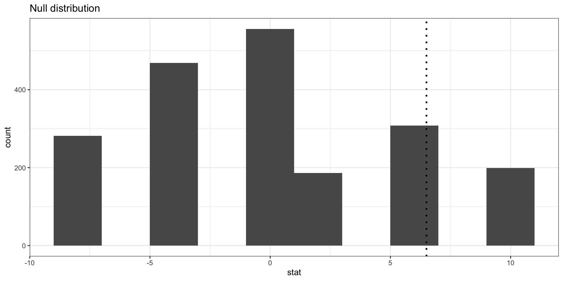
Calculate the p-value

null_dist %>%
  filter(stat > 6.5) %>%
  summarise(p_value = n()/nrow(null_dist))
# A tibble: 1 × 1
  p_value
    <dbl>
1  0.0995

Let’s move on to a real and more interesting example

  • Bertrand and Mullainathan studied racial discrimination in responses to job applications in Chicago and Boston. They sent 4,870 resumes, randomly assigning names associated with different racial groups.

  • Data are in openintro package as an object called resume

  • I will save as myDat

library(openintro)
myDat <- resume 

Call Backs by Race

  • Remember, race of applicant is randomly assigned: the resumes are otherwise identical
mns <- myDat %>% 
  group_by(race) %>% 
  summarize(calls = mean(received_callback))
mns
# A tibble: 2 × 2
  race   calls
  <chr>  <dbl>
1 black 0.0645
2 white 0.0965


Let’s save the means for white and black applicants.


mean_white = mns$calls[2]
mean_black = mns$calls[1]


And calculate the treatment effect. The treatment effect is the difference in means.


teffect <- mean_white - mean_black
teffect
[1] 0.03203285

Is this evidence of racial discrimination?

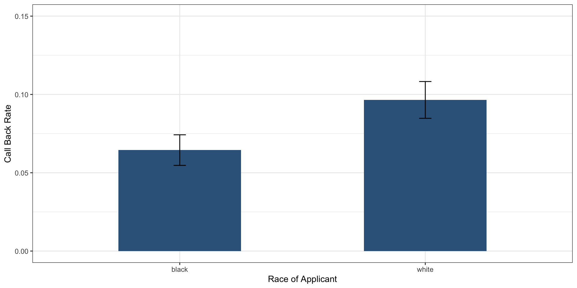
Before formal hypothesis tests, let’s look at the data–the estimates and the confidence intervals…

Esimates and CIs

library(estimatr)
estimates <- resume %>% 
  group_by(race) %>% 
  do(tidy(lm_robust(received_callback ~ 1, data = .))) %>% 
  select(race, estimate, conf.low, conf.high)

Esimates and CIs

estimates
# A tibble: 2 × 4
# Groups:   race [2]
  race  estimate conf.low conf.high
  <chr>    <dbl>    <dbl>     <dbl>
1 black   0.0645   0.0547    0.0742
2 white   0.0965   0.0848    0.108 

What would you conclude and why?

Hypothesis Test


  • What is the null hypothesis?
  • What is the alternative hypothesis?
  • How can we formally test the null hypothesis to decide whether to reject it?

Formal Hypothesis Test


  • Calculate the difference in means (White - Black)
  • Shuffle the race variable randomly (permute the race)
  • Calculate the difference in means for the shuffled data
  • Repeat many times (thousands of times)
  • Simulates the null distribution of differences in callbacks

We can use tidymodels for this

null_dist <- myDat %>%
  specify(response = received_callback, explanatory = race) %>%
  hypothesize(null = "independence") %>%
  generate(5000, type = "permute") %>%
  calculate(stat = "diff in means", 
            order = c("white", "black")) 

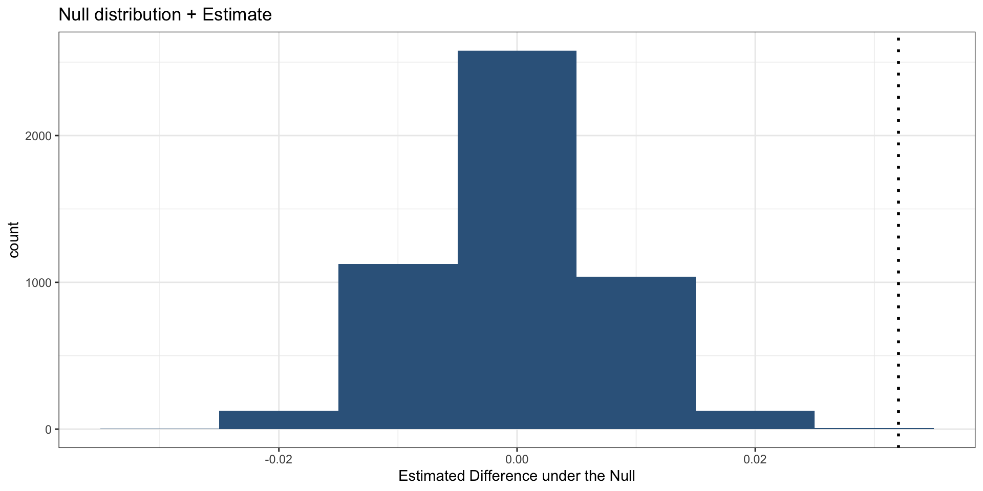
Visualize

Calculate the p-value

null_dist %>%
  filter(stat > teffect) %>%
  summarise(p_value = n()/nrow(null_dist))
# A tibble: 1 × 1
  p_value
    <dbl>
1  0.0002

What should we conclude?


  • The p-value is very small (below .05 threshold)

  • Therefore, we reject the null hypothesis: the racial gap is extremely unlikely to have occurred due to chance alone

  • This is evidence of racial discrimination

Your Tasks

  • Use the gender variable in the resume data to assess whether there is gender discrimination in call backs

    • Plot means and 95% confidence intervals for the call back rate for men and women
    • Write the null and alternative hypotheses
    • Simulate the null distribution
    • Visualize the null distribution and the gender gap
    • Calculate the p-value
  • Challenge problem: Examine gender discrimination separately for those with and without a college degree (using same process as above). [the variable is college_degree]

    • What do you conclude from your data? Here, consider the size of the gender gaps AND the results from the hypothesis test.